Genome-scale Multilocus Sequence Typing CBW Tutorial

Dillon Barker - 12 July 2018

Learning Objectives

Students will learn to:

- Interpret genome-scale MLST results
- Compare different allelic typing methods
- Visualize MLST data with GrapeTree
- Investigate a foodborne outbreak scenario

Dataset Description

Your local Public Health Agency has been tasked with investigating an outbreak of Salmonella enterica. Your bioinformatician has generated some in silico typing results for 200 recent Salmonella enterica clinical isolates, but it will be up to you to perform the downstream analysis.

Setting Up

First, we’ll need to connect slightly differently to our tutorial computers than we have been so far, due to some minor limitations of GrapeTree.

Linux/Mac users:

ssh -L 8080:localhost:8000 -i CBW.pem ubuntu@XX.oicrcbw.ca

Windows users:

• Open PuTTY
  • Under Sessions, load your connection settings
  • In Connection -> SSH -> Tunnels:
    • Type “8080” into Source Port
    • Type “localhost:8000” into Destination
    • Click Add
    • Click Open

Now we can run GrapeTree on the server:

grapetree

And we can view it in your favourite web browser:

localhost:8080

Now transfer the course files to somewhere convenient, such as your Desktop, on your local computer.

Linux/Mac

scp -r -i ~/CBW.pem ubuntu@XX.oicrcbw.ca:CourseData/IDGE_data/module3 ~/Desktop/ 

Windows:

Use WinSCP to connect to the server, and download the files to your local computer.

Exercise 1

Since classical 7-gene Multilocus Sequence Typing (MLST) may be familiar to you, you decide to use that first to investigate the strains that are suspected to belong to the outbreak.

Your bioinformatician has generated the typing data, but she has not visualized the data for you. To view your results in a human-friendly manner, we’ll be using GrapeTree.

In GrapeTree, click Load Files and load ~/workspace/CourseData/mlst_calls.tsv

Hmm - that wasn’t terribly useful. MLST-like systems are limited by both the number of genes in the scheme and the diversity of those genes. Although the classical MLST genes we used are well-curated, there are only seven of them.

Let’s try to use a larger number of genes to distinguish between strains within this outbreak population. Our bioinformatician has also provided typing data for a 290-gene Core Genome Multilocus Sequence Typing scheme.

As before, go to Load Files and this time select cgmlst290_calls.tsv from the same directory. The resulting minimum spanning tree will show much more structure than what was generated by the 7-gene method.

We can show the regions within the much higher resolution cgMLST typing data that correspond to the classical MLST Sequence Types.

Again, click Load Files, this time selecting metadata.tsv.

On the left hand side of the screen, under Tree Layout -> Node Style select ST within the Colour By drop-down menu.

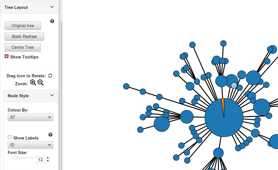
We can also change the colour palette to make differences easier to see.

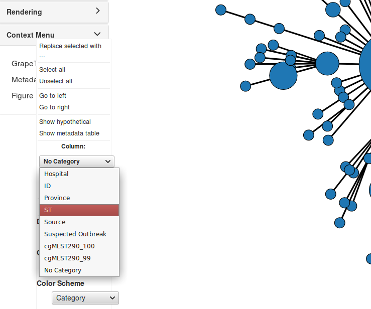
In Context Menu, click on Metadata. In the Column drop-down menu select ST as the column you wish to recolour, and in the Color Scheme drop-down, select Category 2.

The cgMLST calls given to us by our bioinformatician were defined to be highly portable across this species. In addition to this, we were also given the typing results for an ad hoc Whole Genome Multilocus Typing scheme. This scheme is valid only for this particular set of strains, but it allows us a higher resolution look at the structure of the given population.

As above, let’s load the wgMLST calls from the file wgmlst2359_calls.tsv, and then load metadata.tsv once again, as GrapeTree resets this information when new calls are loaded.

There’s a lot of information here. We can cluster the data back into useful groups.

Within the provided metadata, try projecting cgMLST clusters generated at 100% and 99% thresholds. Also, try adjusting the Collapse Branches parameter found in Tree Layout -> Branch Style

Questions:

- How does varying the number of loci in a MLST scheme affect the results
  we see?
- What's the difference between a higher resolution method clustered at
  <100% identity and a lower resolution method clustered at 100%?

Exercise 2

It’s also possible to project provenance or metadata on our population as well. This will be helpful for investigating this outbreak.

We have two major classes of epidemiological metadata available to us: whether strains are believed to belong to the outbreak, and the source of infection if known.

Try projecting the Outbreak data first. This column tells us whether each strain is suspected to belong to the outbreak or not.

You can also project Source information. Display the Source information using the workflow you’ve practiced.

Let’s derive a new metadata field using a few lines of R.

Open R in your terminal on the teaching computer:

R

# Load the read-only metadata file
metadata <- read.table('~/CourseData/IDGE_data/module3/metadata.tsv'
                       sep = '\t',
                       header = TRUE)

# Create the derivate metadata field
metadata$Source_Outbreak <- paste(metadata$Source,
                                  metadata$Outbreak,
                                  sep = '-')

# Note the new filepath to your edited metadata file
write.table(metadata,
            file = '~/workspace/metadata_extra_field.tsv',
	    row.names = FALSE,
            quote = FALSE,
            sep = '\t')

quit()

Now use scp or WinSCP to transfer ~/workspace/metadata_extra_field.tsv to your local computer, just like the beginning of this tutorial.

We can visualize this new derivative metadata field by re-loading our metadata file.

- Click **Load Files**
- Select **metadata_extra_field.tsv** from to reload the file with the new values

Questions:

- Can you speculate as to the source of the outbreak?
- What is the distribution of strains in the outbreak?
- Are there strains that were putatively part of the outbreak that you
  don't think should be included? Are there outbreak strains that were
  excluded?
- What is the distance between the main clades of the outbreak?

Exercise 3

You’re not expected to run the following code during class. However, you may choose to run through this later.

The following represents some of the basic steps that the bioinformatician took to prepare data for you to use in the above scenario.

conda create -n cbw_analysis -c bioconda shovill

conda activate cbw_analysis

pip3 install chewbbaca

mkdir assemblies genomes

for base in $(basename -a -s .fastq.gz fastqs/*.fastq.gz | cut -d'_' -f 1 | uniq); do

    shovill --R1 ${base}_1.fastq.gz \
            --R2 ${base}_2.fastq.gz \
            --clip \
            --outdir assemblies/${base}

    ln -sr assemblies/${base}/contigs.fa genomes/${base}.fasta

done


chewBBACA.py CreateSchema -i genomes/ -o wgmlst --cpu 4

chewBBACA.py AlleleCall -i genomes/ -g wgmlst/ -o wgmlst/

chewBBACA.py ExtractCgMLST -i wgmlst/AlleleCalls.tsv -o cgmlst