CBW-IMPACTT Microbiome Analysis Module 5 Lab

CBW IMPACTT Workshop

Kevin Muirhead and Dr. Laura Sycuro

Module 5: Metagenomic Assembly and Metagenome Assembled Genomes Tutorial

The purpose of this tutorial is to introduce common bioinformatics tools for processing metagenomics datasets using an assembly-based approach and binning to produce metagenome assembled genomes (MAGs). You will be taken through each step of the process with a focus on developing conceptual understanding, identifying key parameters, evaluating data quality, and weighing analytical choices. For this tutorial we will be using four vaginal metagenomes generated in a pilot study of baseline samples (N=17) from participants in the Kenyan Girls Health Study (Sycuro lab). This longitudinal cohort study enrolled adolescent girls and young women (AGYW) aged 16–20 years old from Thika, Kenya to study drivers of Lactobacillus dominance. A healthy vaginal microbiome is dominated by a single Lactobacillus species, such as L. crispatus or L. iners, which can make up anywhere from 50% to >90% of the total bacterial load. In contrast, a dysbiotic vaginal microbiome is characterized by a high diversity of anaerobic bacteria such as Gardnerella vaginalis. This dataset will introduce you to some of these species once you annotate and classify the samples’ MAGs.

This dataset has been previously processed through a quality control and filtering pipeline that ensures that sequencing adapters are removed, read ends are trimmed to remove bases with low quality base calls, reads that are too short or exhibiting overall low quality are removed, and reads aligning to the human genome are removed. The pipeline we utilize for quality filtering and host decontamination is freely available to the public (https://github.com/SycuroLab/metqc), though many well-established/stand-alone tools are available.

Our objective today is to guide you through the commands used in the three analytical steps introduced during the lecture: 1) Assembly; 2) Binning; and 3) Annotation. There are many steps involved in metagenome assembly and binning that are computationally demanding, often taking several hours to several days on a high-performance computing (HPC) node, depending on the size of the dataset. The provided datasets are relatively compact – representing typical shallow shotgun metagenomes – but some steps still took up to 30 min to complete on a HPC node with 14 or 28 threads and up to 50GB RAM or higher. A server such as the AWS instance with 8 threads and 16GB RAM will take much longer to complete and some jobs may not complete at all. Thus, we have completed each step beforehand and provided the output files so that you can follow along and only carry out some of the less computationally intensive steps on your own.

Each step that you will perform on your AWS instance in class is highlighted in gray. Procedural notes are indented and italicized and critical warnings are bolded. If you wish to skip directly to the working component of the tutorial, go to page 3.

Overview of the Dataset and Workflow

The KGHS dataset was downloaded from NCBI BioProject PRJNA838641 (Table 1). Please see Appendix 1 for more information on how this was performed and how to download public datasets using the NCBI SRA toolkit program fasterq-dump.

Table 1: Dataset information.

Sample Name	SRA Run ID	Total Number of Cleaned Reads	Read Length	File Size
KGHS_1-0	SRR19237623	1321174	2x150	2x370MB
KGHS_8-0	SRR19237609	3773184	2x150	2x1.3GB
KGHS_9-0	SRR19237608	1116676	2x150	2x450MB
KGHS_15-0	SRR19237617	3701058	2x150	2x1.3GB

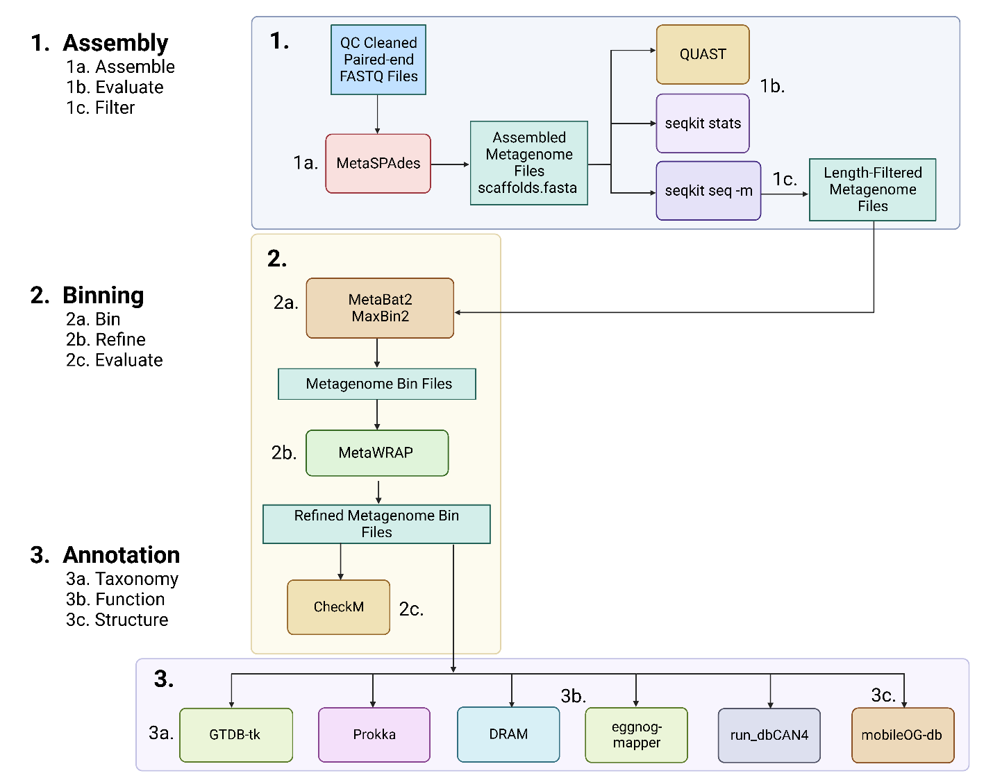
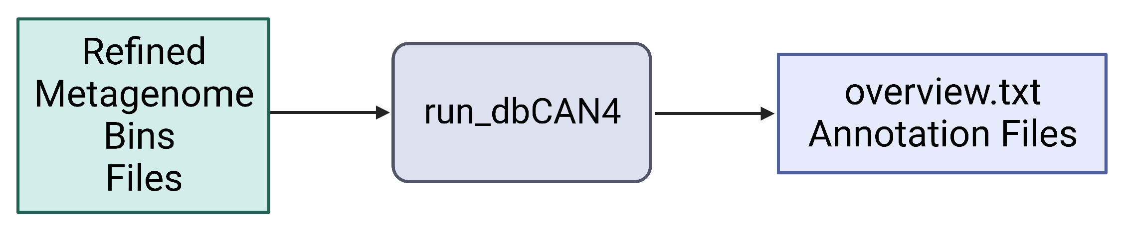
Figure 1: Overview of the assembly, binning, and annotation workflow.

Section 1: Assembly

Make the directory for the mags_workshop.

mkdir -p /home/ubuntu/workspace/mags_workshop

To get started please use a symbolic link to point your CourseData files to the workspace folder.

ln -s /home/ubuntu/CourseData/MIC_data/mags_workshop/module5 /home/ubuntu/workspace/mags_workshop/module5

change your directory to the module5 folder for this workshop using the following command;

cd /home/ubuntu/workspace/mags_workshop/module5

Step 1a: Assemble metagenomic reads using MetaSPAdes

SPAdes (https://github.com/ablab/spades)

SPAdes assembles genomes and metagenomes[1]. The metaspades.py command is used to run MetaSPAdes, the version designed to operate on metagenomic datasets.

The -k flag allows for a wider range of kmers to be used, which helps to find the most optimal assembly. We are using the following kmer values: -k 21,33,55,77,99,127. Must be odd numbers from 21 to 127. The paper used the default settings for kmer values: -k 21,33,55.

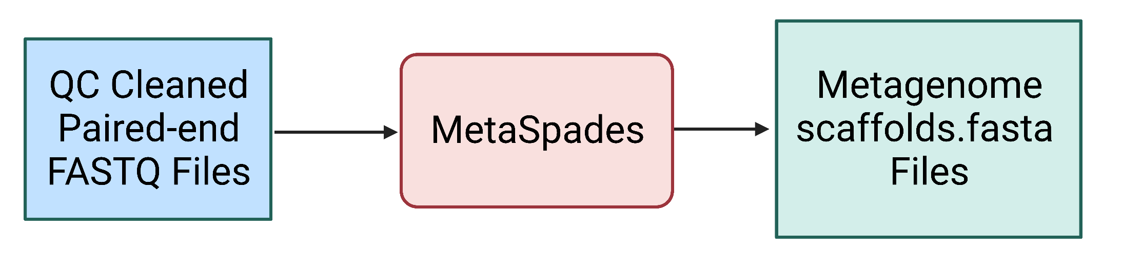
Figure 2. The MetaSPAdes step uses the quality control cleaned paired end FASTQ files as input and generates a number of output files, including the scaffolds.fasta file containing all scaffold sequences for the metagenomic assembly.

WARNING: DO NOT RUN MetaSPAdes!

Notes: For a dataset this size (~300MB – 1.3GB per read1.fastq and read2.fastq), with 28 threads, MetaSPAdes ran for 17 – 27 minutes using 13.2GB – 17.6GB. A larger metagenome (20 GB) will typically take several hours to several days using these parameters. The AWS instance may similarly take many hours to complete if you attempt to assemble these data on it. For the purpose of the in-class tutorial, the output files are provided for you to view:

cd /home/ubuntu/workspace/mags_workshop/module5/output/metagenome_assemblies/KGHS_1-0

We have also provided a conda environment and commands within shell scripts to run MetaSPAdes, with more details in Appendix 2.

Example commands for sample KGHS_1-0:

# Change the directory back to the module5 directory.

cd /home/ubuntu/workspace/mags_workshop/module5

# Activate the SPAdes conda environment so that you can run MetaSPAdes.

conda activate spades_env

# Execute the MetaSPAdes command using kmer lengths 21,33,55,77,99,127 to find the optimized assembly with 28 threads and 50GB RAM.

metaspades.py -k 21,33,55,77,99,127 -t 28 -m 50 -o metagenome_assemblies/KGHS_1-0 -1 cleaned_fastq_files/KGHS_1-0_1.fastq -2 cleaned_fastq_files/KGHS_1-0_2.fastq

MetaSPAdes output: contains many output files, the log file, and intermediate file directories.

Key output files:

contigs.fasta - The FASTA file containing the assembled metagenomic contigs

less /home/ubuntu/workspace/mags_workshop/module5/output/metagenome_assemblies/KGHS_1-0/contigs.fasta

scaffolds.fasta - The FASTA file containing the assembled metagenomic scaffolds

less /home/ubuntu/workspace/mags_workshop/module5/output/metagenome_assemblies/KGHS_1-0/scaffolds.fasta

spades.log – The log text file containing information on what the program did, how long each step took, and where things went wrong (if they do).

less /home/ubuntu/workspace/mags_workshop/module5/output/metagenome_assemblies/KGHS_1-0/spades.log

Step 1b: Evaluate assembly quality using QUAST

QUAST (https://github.com/ablab/quast)

QUAST is a program that generates assembly quality metrics[2]. It allows for a quick check of the success of your metagenomic assembly and comparisons with different assembly parameters (such as -k values) or algorithms (such as IBDA-UD[3] or MEGAHIT[4]).

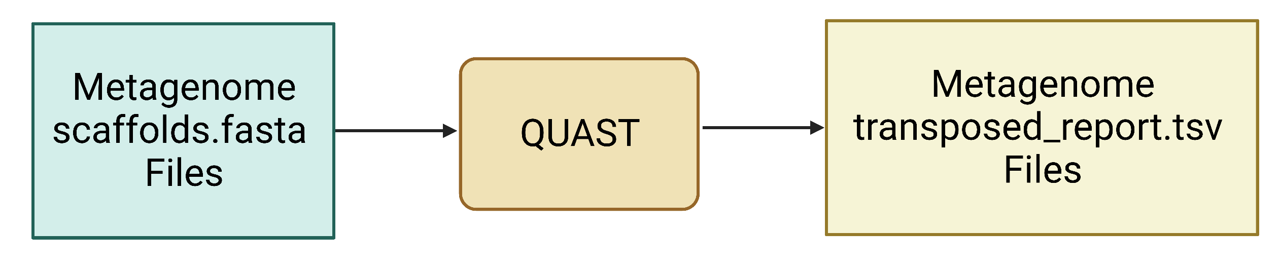
Figure 3. QUAST uses assembled contig or scaffold FASTA files as input and generates a number of output files, including the transposed_report.tsv file.

Example commands for sample KGHS_1-0:

# Change the directory back to the module5 directory.

cd /home/ubuntu/workspace/mags_workshop/module5

# Activate the QUAST conda environment.

conda activate quast_env

# Run QUAST on the contigs.fasta file.

quast.py --output-dir metagenome_assemblies/KGHS_1-0/quast_contigs --threads 1 output/metagenome_assemblies/KGHS_1-0/contigs.fasta

# Run QUAST on the scaffolds.fasta file.

quast.py --output-dir metagenome_assemblies/KGHS_1-0/quast_scaffolds --threads 1 output/metagenome_assemblies/KGHS_1-0/scaffolds.fasta

Example output:

QUAST contigs.fasta

less /home/ubuntu/workspace/mags_workshop/module5/metagenome_assemblies/KGHS_1-0/quast_contigs/transposed_report.tsv

QUAST scaffolds.fasta

less /home/ubuntu/workspace/mags_workshop/module5/metagenome_assemblies/KGHS_1-0/quast_scaffolds/transposed_report.tsv

Table 2: QUAST evaluation metrics for contigs.fasta and scaffolds.fasta

Assembly	Number of Contigs	Largest Contig	Total Length	GC (%)	N50	# N’s per 100 kbp
Contigs	29757	256891	5998229	36.61	28084	0
Scaffolds	29708	256891	6021946	36.64	29877	33.54

Step 1c: Filter scaffolds <1500 nt and evaluate change in assembly quality using seqkit

seqkit (https://github.com/shenwei356/seqkit)

seqkit will be used to filter the scaffolds[5], retaining those with a minimum length of 1500 nt.

Most binning software recommends using 1500 nt scaffolds as the default. You can try using 2000 and 2500 to see how the resulting bins compare on your own time.

WARNING: Using scaffolds shorter than 1500 nt will result in the tetranucleotide frequencies becoming poorly represented, yielding low quality MAGs.

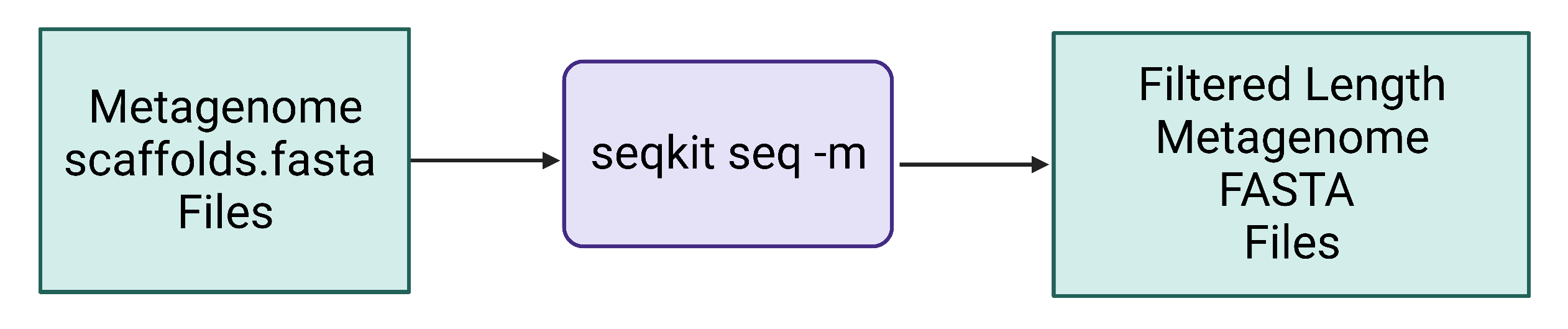
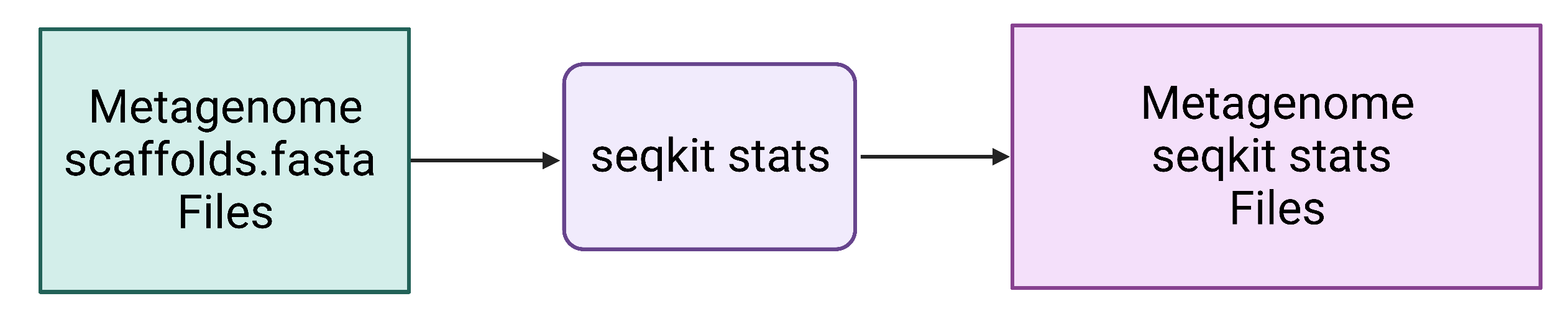
Figure 4. Seqkit seq uses assembled contig or scaffold FASTA files as input and generates a new length-filtered contig or scaffold FASTA file. Seqkit stats quickly/easily reports quality metrics and will be applied to the original scaffolds.fasta file and the length-filtered KGHS_1-0_min1500.fasta file to compare them.

Example commands for sample KGHS_1-0:

# Change the directory back to the module5 directory.

cd /home/ubuntu/workspace/mags_workshop/module5

# Create the seqkit conda environment.

conda create --name seqkit_env

# Activate the seqkit conda environment.

conda activate seqkit_env

# Install the seqkit conda package.

conda install -c bioconda seqkit

# Create the filtered_metagenomes/KGHS_1-0 directory.

mkdir -p filtered_metagenomes/KGHS_1-0

# Filter scaffolds to a minimum length of 1500 nt.

seqkit seq -m 1500 output/metagenome_assemblies/KGHS_1-0/scaffolds.fasta > filtered_metagenomes/KGHS_1-0/KGHS_1-0_min1500.fasta

# Run seqkit stats on the KGHS_1-0 contigs.fasta file.

seqkit stats -a output/metagenome_assemblies/KGHS_1-0/contigs.fasta > metagenome_assemblies/KGHS_1-0/contigs.fasta.seqkit.stats.txt

Example output:

# Run seqkit stats on the KGHS_1-0 scaffolds.fasta file.

seqkit stats -a output/metagenome_assemblies/KGHS_1-0/scaffolds.fasta > metagenome_assemblies/KGHS_1-0/scaffolds.fasta.seqkit.stats.txt

Example output:

# Run seqkit with the stats option on the length-filtered KGHS_1-0_min1500.fasta file to see how filtering affected the minimum length reported and the number of scaffolds.

seqkit stats -a output/filtered_metagenomes/KGHS_1-0/KGHS_1-0_min1500.fasta > filtered_metagenomes/KGHS_1-0/KGHS_1-0_min1500.fasta.seqkit.stats.txt

Example output:

Section 2: Binning

Step 2a: Bin scaffolds using at least 2 different algorithms

Assembled scaffolds will be binned using two binning algorithms: MetaBAT2[6] and MaxBin2[7]. Tetranucleotide frequency and abundance (coverage) will be the scaffold attributes used by both algorithms.

You can read the following paper for more information and a comprehensive comparison of softwares for binning/bin refinement: (https://bmcbioinformatics.biomedcentral.com/articles/10.1186/s12859-020-03667-3#Sec2)

Figure 5. Length-filtered scaffold FASTA files are provided as input for binning softwares such as MetaBat2 and MaxBin2. Read mapping files (.bam) are also provided as input to the binning softwares. The outputs of binning are smaller FASTA files, one for each bin. These are in turn provided as input in the bin refinement step, producing the optimal set of non-redundant bin FASTA files.

bwa (https://github.com/lh3/bwa)

samtools (http://www.htslib.org)

To generate the sample abundance data (a correlate of depth of coverage) required by the binning algorithms, the clean paired end reads from each sample have to be mapped to the assembled metagenome (1500 nt+ scaffolds only). We used BWA[8] and samtools[9] to map the reads back to the filtered metagenome.

WARNING: DO NOT RUN BWA mem or samtools

The mapping step takes a few minutes using 14 threads.

Example commands for sample KGHS_1-0:

# Change the directory back to the module5 directory.

cd /home/ubuntu/workspace/mags_workshop/module5

# Activate the bwa conda environment.

conda activate bwa_env

# Create an index of the filtered scaffolds using bwa index.

bwa index filtered_metagenomes/KGHS_1-0/KGHS_1-0_min1500.fasta

# Map the paired end reads from sample KGHS_1-0 to the filtered scaffolds using bwa mem.

bwa mem -t 4 filtered_metagenomes/KGHS_1-0/KGHS_1-0_min1500.fasta cleaned_fastq_files/KGHS_1-0_1.fastq cleaned_fastq_files/KGHS_1-0_2.fastq > filtered_metagenomes/KGHS_1-0/KGHS_1-0.sam

# Activate the samtools conda environment.

conda activate samtools_env

# Sort the sam file and convert to bam using samtools.

samtools sort -@ 4 -O BAM -o filtered_metagenomes/KGHS_1-0/KGHS_1-0.bam filtered_metagenomes/KGHS_1-0/KGHS_1-0.sam

MetaBat2 (https://bitbucket.org/berkeleylab/metabat/src/master/)

MaxBin2 (https://sourceforge.net/projects/maxbin2/)

Example commands for sample KGHS_1-0:

Bin length-filtered scaffolds using MetaBat2.

# Change the directory back to the module5 directory.

cd /home/ubuntu/workspace/mags_workshop/module5

# Activate the metabat2 conda environment.

conda activate metabat2_env

# Create the initial binning KGHS_1-0 output directory.

mkdir -p initial_binning/KGHS_1-0/

# Generate the metabat2 depth of coverage text file using the bam file generated in the mapping step.

jgi_summarize_bam_contig_depths --outputDepth initial_binning/KGHS_1-0/metabat2_depth.txt output/filtered_metagenomes/KGHS_1-0/KGHS_1-0.bam

# Create the initial binning working directory for metabat2.

mkdir -p initial_binning/KGHS_1-0/working_dir/metabat2 

# Run metabat2 on the filtered scaffolds using the metabat2 depth of coverage file.

metabat2 -i output/filtered_metagenomes/KGHS_1-0/KGHS_1-0_min1500.fasta -a initial_binning/KGHS_1-0/metabat2_depth.txt -o initial_binning/KGHS_1-0/working_dir/metabat2/KGHS_1-0_bin -m 1500 -t 1 –unbinned

# Create the initial binning metabat2 directory for the KGHS_1-0 sample.

mkdir -p initial_binning/KGHS_1-0/metabat2

# Copy the metabat2 bins to the initial binning metabat2 directory.

cp initial_binning/KGHS_1-0/working_dir/metabat2/KGHS_1-0_bin.[0-9]*.fa initial_binning/KGHS_1-0/metabat2

Bin length-filtered scaffolds using MaxBin2.

# Activate the metabat2 conda environment for running the jgi_summarize_bam_contig_depths program from the metabat2 software to generate the depth of coverage file for maxbin2.

conda activate metabat2_env

# Generate the maxbin2 depth of coverage text file using the bam file generated in the mapping step.

jgi_summarize_bam_contig_depths --outputDepth initial_binning/KGHS_1-0/KGHS_1-0_maxbin2_depth.txt --noIntraDepthVariance output/filtered_metagenomes/KGHS_1-0/KGHS_1-0.bam

# Create the maxbin2 abundance file using the first and third columns of the maxbin2 depth of coverage file.

tail -n+2 initial_binning/KGHS_1-0/KGHS_1-0_maxbin2_depth.txt | cut -f1,3 > initial_binning/KGHS_1-0/KGHS_1-0_maxbin2_abund.txt

# Print the path of the maxbin2 abundance file to a list file.

echo initial_binning/KGHS_1-0/KGHS_1-0_maxbin2_abund.txt > initial_binning/KGHS_1-0/KGHS_1-0_maxbin2_abund_list.txt

# Activate the maxbin2 conda environment.

conda activate maxbin2_env

# Create the working maxbin2 output directory.

mkdir -p initial_binning/KGHS_1-0/working_dir/maxbin2

# Run MaxBin2 using the filtered scaffolds fasta file and the maxbin2 abundance list.

perl software_dir/MaxBin-2.2.7/run_MaxBin.pl -contig output/filtered_metagenomes/KGHS_1-0/KGHS_1-0_min1500.fasta -markerset 107 -thread 14 -min_contig_length 1500 -out initial_binning/KGHS_1-0/working_dir/maxbin2/KGHS_1-0_bin -abund_list initial_binning/KGHS_1-0/KGHS_1-0_maxbin2_abund_list.txt

# Create the maxbins2 output directory so we can rename the bins; this is needed in order for metawrap to use them as input.

mkdir -p initial_binning/KGHS_1-0/maxbin2

# Rename bins and copy the maxbin2 bins to the maxbin2 bin directory.

for bin_file in $(ls initial_binning/KGHS_1-0/working_dir/maxbin2 | grep "\.fasta");

do echo $bin_file;

filename=$(basename $bin_file '.fasta');

bin_num=$(echo $filename | sed -r "s/KGHS_1-0_bin\\0+//g");

echo $bin_num;

new_filename="KGHS_1-0_bin.${bin_num}.fa";

echo $new_filename;

cp initial_binning/KGHS_1-0/working_dir/maxbin2/$bin_file initial_binning/KGHS_1-0/maxbin2/$new_filename;

done

Example output:

Table 3: The number and quality of the initial bins from MetaBAT2 and MaxBin2.

Bin ID	Binning Program	Number of contigs	Completeness	Contamination	GC	Lineage	N50	Total Size
bin.1	MetaBAT2	31	73.08	0	0.34	Lactobacillus	70417	1018998
bin.2	MetaBAT2	9	44.82	0	0.321	Bacteria	82317	399990
bin.3	MetaBAT2	4	12.5	0	0.325	root	154219	296894
bin.4	MetaBAT2	71	55.17	1.724	0.363	Bacteria	22949	1213585
bin.5	MetaBAT2	23	4.166	0	0.377	root	16390	295846
bin.6	MetaBAT2	18	20.34	0	0.379	Lactobacillus	19069	239066
bin.7	MetaBAT2	22	11.44	0	0.336	Bacteria	40251	519230
bin.1	MaxBin2	136	79.06	0.216	0.373	Lactobacillus	17642	1593681
bin.2	MaxBin2	72	98.96	11.9	0.329	Lactobacillus	84766	1639119
bin.3	MaxBin2	75	98.83	0.322	0.341	Lactobacillus	67177	1711736

You can see that there are quite a few bins being generated using MetaBAT2 and MaxBin2 with variable number of contigs, N50 and total sizes. Each has its own completeness and contamination values from CheckM that is used to evaluate the bins. The percent completeness is the proportion of universal single copy marker genes present in the bin and percent contamination is the proportion of contamination from other genomes in your bin. You can see that the lineage is down to the genus level for some. That is the lowest taxonomy you can get out of using CheckM and will need to use GTDB-tk once you have MAGs. The quality of bins are important when moving forward and you can use metawrap to refine your bins into higher quality bins.

Step 2b: Refine bins using metaWRAP’s bin refinement module

metaWRAP bin_refinement module (https://github.com/bxlab/metaWRAP)

MetaWRAP uses CheckM[10] and Binning_refiner[11] to optimize the quality of bins. It takes up to 3 different sets of bins at a time. Since you are using two binning algorithms, you will specify the -A and -B parameter options. If you used a third, you would add the -C option.

WARNING: DO NOT RUN MetaWRAP!

Since MetaWRAP uses CheckM and it takes quite a bit of time to complete. We precomputed the refined bins taking 31 minutes using 28 threads and 34 GB.

Example commands for sample KGHS_1-0 bins:

# Change the directory back to the module5 directory.

cd /home/ubuntu/workspace/mags_workshop/module5

# Start the conda environment for MetaWRAP bin_refinement.

conda activate metawrap_bin_refinement_env

# Create the bin_refinement directory.

mkdir -p bin_refinement/KGHS_1-0

# Run the metawrap bin refinement module.

metawrap bin_refinement -o bin_refinement/KGHS_1-0 -t 1 -A initial_binning/KGHS_1-0/metabat2 -B initial_binning/KGHS_1-0/maxbin2 -c 50 -x 10

Example output:

The statistics file outlining the results of the MetaWRAP bin refinement module.

less /home/ubuntu/workspace/mags_workshop/module5/output/bin_refinement/KGHS_1-0/metawrap_50_10_bins.stats

Table data obtained from the MetaWRAP bin refinement module statistics output file and QUAST transposed_report.tsv output file for KGHS_1-0_bin.1 and KGHS_1-0_bin.3.

Table 4: Number and quality of bins refined using MetaWRAP.

Bin ID	Bin Refining Program	Number of Contigs	Largest Contig	Complete-ness	Contam-ination	Total Length	GC (%)	N50
KGHS_1-0_bin.1	MetaWRAP	75	133687	98.83	0.341	1711736	34.19	67177
KGHS_1-0_bin.3	MetaWRAP	136	59107	76.06	0.373	1593681	37.33	17642

Step 2c: Evaluate bin quality using CheckM

You will now evaluate the quality of your bins to determine which are suitable for downstream analyses as metagenome assembled genomes (MAGs).

CheckM requires a larger amount of RAM because of pplacer. We ran the checkm command prior to this tutorial because it takes 13 mins using 14 threads and 30 GB RAM per MAG.

CheckM (https://github.com/Ecogenomics/CheckM)

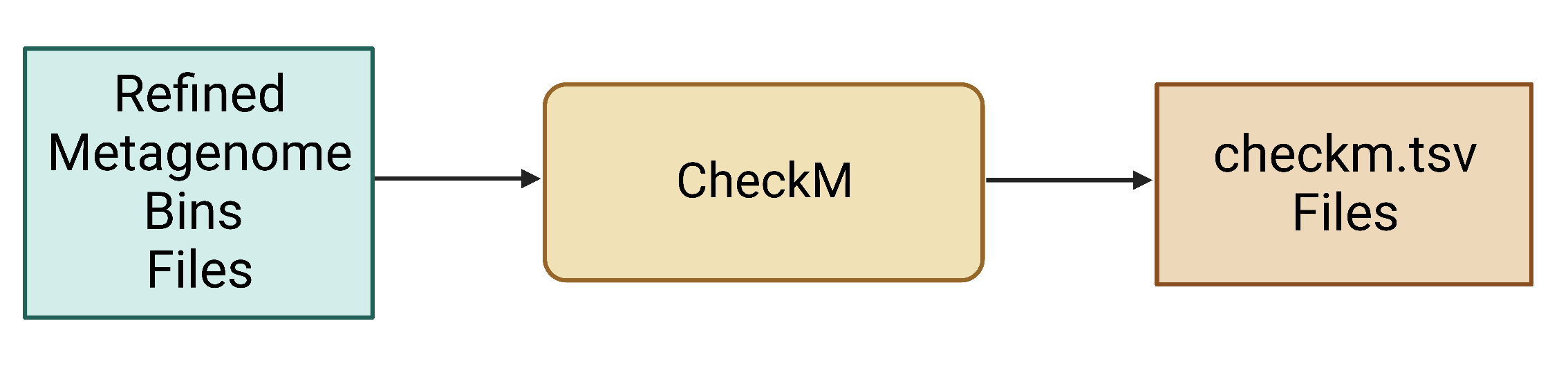
Figure 6. Refined bin FASTA files are provided as input for CheckM, which produces a variety of output files, including different .tsv files that contain various data summaries. Note that some .tsv files may not be produced unless specified using the appropriate parameter.

WARNING: Do not run CheckM!

This was run prior to the tutorial, taking 13 min per MAG using 14 threads and 30GB RAM. It will run into memory issues using the AWS instance since it requires more than 16GB of memory.

WARNING: Before running CheckM you need to set the path to the CheckM database. If you don’t set the database, or lack proper user permissions to read the database, CheckM will print an error message until you run out of disk space.

Example commands for the KGHS_1-0.bin1.fa MAG:

# Change the directory back to the module5 directory.

cd /home/ubuntu/workspace/mags_workshop/module5

# Set the CheckM database path.

echo “software_dir/checkm_data_dir”

checkm data setRoot

# Create the checkm directory.

mkdir -p refined_bins/KGHS_1-0/KGHS_1-0_bin.1/checkm

# Copy the bin and rename to KGHS_1-0.bin1 so that we can run CheckM.

cp bin_refinement/KGHS_1-0/metawrap_50_10_bins/bin.1.fa refined_bins/KGHS_1-0/KGHS_1-0_bin.1/checkm/KGHS_1-0_bin.1.fa

# Activate the CheckM conda environment.

conda activate checkm_env

# Run CheckM to assess the quality of the KGHS_1-0.bin1.fa MAG.

checkm lineage_wf -t 14 -x fa –tab_table –file refined_bins/KGHS_1-0/KGHS_1-0_bin.1/checkm/checkm.tsv refined_bins/KGHS_1-0/KGHS_1-0_bin.1/checkm refined_bins/KGHS_1-0/KGHS_1-0_bin.1/checkm

Example output:

less /home/ubuntu/workspace/mags_workshop/module5/output/refined_bins/KGHS_1-0/KGHS_1-0_bin.1/checkm/checkm.tsv

These are the most important columns from CheckM.

Bin Id – The ID of the MAG.

# genomes – Number of genomes predicted in the MAG.

Completeness – The percent of universal single copy marker genes present in the MAG.

Contamination – The percent of contamination found in your MAG.

WARNING: CheckM does not provide an accurate taxonomic classification of the MAGs – do not consider what is reported by this program as the final assignment. GTDB-tk gives a more accurate classification (Section 3, Step 3a below).

Exercise:

# Change the directory to the checkm bin directory.

cd /home/ubuntu/workspace/mags_workshop/module5/output/refined_bins/KGHS_1-0/KGHS_1-0_bin.1/checkm

# Use awk to filter the CheckM results using >= 50% completeness and <=10 % contamination.

awk -F'\t' '(($12 >= 50) && ($13 <= 10)){print $0}' <(tail -n+2 < checkm.tsv) > checkm_output_ge50comp_le10contam.tsv

# Use less to view the CheckM results using >= 90% completeness and <=10 % contamination.

less /home/ubuntu/workspace/mags_workshop/module5/output/refined_bins/KGHS_1-0/KGHS_1-0_bin.1/checkm/checkm_output_ge50comp_le10contam.tsv

# Use awk to filter the CheckM results using >= 90% completeness and <=10 % contamination.

awk -F'\t' '(($12 >= 90) && ($13 <= 10)){print $0}' <(tail -n+2 < checkm.tsv) > checkm_output_ge90comp_le10contam.tsv

# Use less to view the CheckM results using >= 90% completeness and <=10 % contamination.

less /home/ubuntu/workspace/mags_workshop/module5/output/refined_bins/KGHS_1-0/KGHS_1-0_bin.1/checkm/checkm_output_ge50comp_le10contam.tsv

Section 3: Annotation

For the purposes of this tutorial, you will consider refined bins with >= 90% completeness and <= 10% contamination (CheckM) as MAGs suitable for downstream annotation.

Step 3a: Classify the taxonomy of each MAG using GTDB-tk

GTDB-tk (https://github.com/Ecogenomics/GTDBTk)

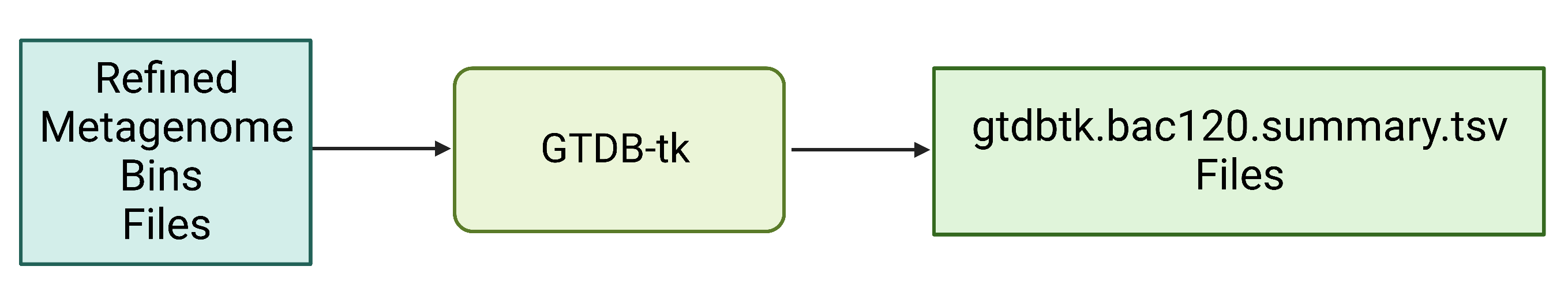
Figure 7. Refined bin FASTA files are provided as input for GTDB-tk, which produces a summary .tsv file with the full taxonomic string and other information about the annotation process.

GTDB-tk is used to classify the taxonomy of your MAGs[12]. If you give GTDB-tk a heavily contaminated MAG or metagenomic assembly, it will fail.

WARNING Do not run GTDB-tk! Note It requires pplacer and will take 20 mins using 46 GB RAM and 14 threads.

Example commands for the KGHS_1-0.bin1.fa MAG:

# Change the directory back to the module5 directory.

cd /home/ubuntu/workspace/mags_workshop/module5

# Activate the gtdbtk conda environment.

conda activate gtdbtk_env

# How to download the database on your own server or local machine. The GTDB-tk database is not installed on the AWS student instance. GTDB-Tk requires ~84G of external data that needs to be downloaded and unarchived.

wget https://data.gtdb.ecogenomic.org/releases/latest/auxillary_files/gtdbtk_data.tar.gz

# Uncompress the tar archive using the tar xvzf command.

tar xvzf gtdbtk_data.tar.gz

# Export the location of the gtdbtk database after it is installed. Change the path to the location of the GTDB-tk database.

export GTDBTK_DATA_PATH=”/path/to/release207_v2”

# Create the gtdbtk directory.

mkdir -p refined_bins/KGHS_1-0/KGHS_1-0_bin.1/gtdbtk

# Copy the KGHS_1-0_bin.1.fa MAG to the gtdbtk directory.

cp bin_refinement/KGHS_1-0/metawrap_50_10_bins/bin.1.fa refined_bins/KGHS_1-0/KGHS_1-0_bin.1/gtdbtk/KGHS_1-0_bin.1.fa

# Run the gtdbtk command on the KGHS_1-0_bin.1.fa MAG

gtdbtk classify_wf –genome_dir refined_bins/KGHS_1-0/KGHS_1-0_bin.1/gtdbtk –extension “fa” –cpus 14 –out_dir refined_bins/KGHS_1-0/KGHS_1-0_bin.1/gtdbtk

Example output:

less /home/ubuntu/workspace/mags_workshop/module5/output/refined_bins/KGHS_1-0/KGHS_1-0_bin.1/gtdbtk/gtdbtk.bac120.summary.tsv

user_genome – The ID of the MAG.

classification – The GTDB-tk taxonomy classification of the MAG.

Question: What is the taxonomy of this MAG?

Step 3b: Annotate the genes in each MAG using Prokka

During the in-class tutorial you will call open reading frames and annotate gene functions using Prokka. Prokka is a quick annotation pipeline that only uses a fraction of the databases that more comprehensive pipelines like DRAM use.

Prokka (https://github.com/tseemann/prokka)

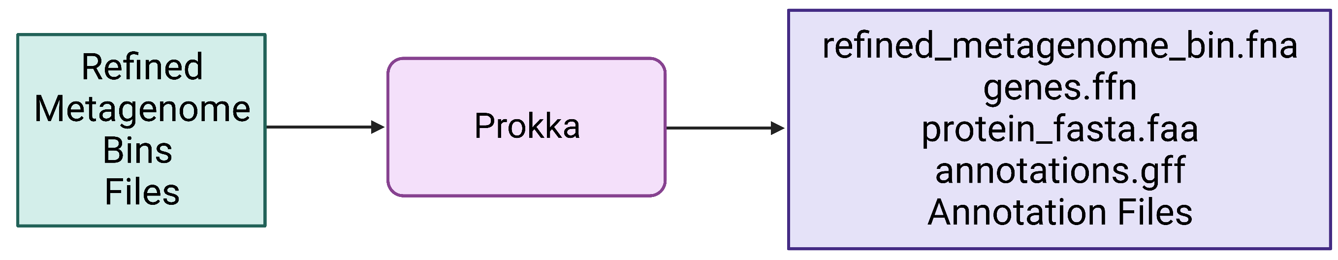
Figure 7. Refined bin FASTA files are provided as input for Prokka, which produces a variety of output files, including gene and protein multi-FASTA files.

Example command for the KGHS_1-0.bin1.fa MAG:

# Change the directory back to the module5 directory.

cd /home/ubuntu/workspace/mags_workshop/module5

# Activate the conda environment.

conda activate prokka_env

# Create the prokka bin directory.

mkdir -p refined_bins/KGHS_1-0/KGHS_1-0_bin.1/prokka

# Rename and copy the KGHS_1-0_bin.1.fa MAG to the refined_bins KGHS_1-0_bin.1 prokka directory.

cp output/bin_refinement/KGHS_1-0/metawrap_50_10_bins/bin.1.fa refined_bins/KGHS_1-0/KGHS_1-0_bin.1/prokka/KGHS_1-0_bin.1.fa

# Run prokka on the KGHS_1-0_bin.1.fa MAG.

prokka --metagenome --outdir refined_bins/KGHS_1-0/KGHS_1-0_bin.1/prokka --prefix KGHS_1-0_bin.1 refined_bins/KGHS_1-0/KGHS_1-0_bin.1/prokka/KGHS_1-0_bin.1.fa --cpus 14 --rfam 1 --force Example output:

KGHS_1-0_bin.1.ffn – The annotated genes FASTA file containing rRNAs, tRNAs, CDS, ncRNAs, etc.

less /home/ubuntu/workspace/mags_workshop/module5/output/refined_bins/KGHS_1-0/KGHS_1-0_bin.1/prokka/KGHS_1-0_bin.1.ffn

KGHS_1-0_bin.1.faa – The protein FASTA file annotated CDS gene sequences translated to proteins.

less /home/ubuntu/workspace/mags_workshop/module5/output/refined_bins/KGHS_1-0/KGHS_1-0_bin.1/prokka/KGHS_1-0_bin.1.faa

KGHS_1-0_bin.1.gff – The generic feature format (GFF) file that contains all the annotated MAG sequence information including start and end position, reading frame, functional annotation, annotation description, etc.

less /home/ubuntu/workspace/mags_workshop/module5/output/refined_bins/KGHS_1-0/KGHS_1-0_bin.1/prokka/KGHS_1-0_bin.1.gff

DRAM (https://github.com/WrightonLabCSU/DRAM)

Although you will not execute DRAM as part of the in-class tutorial, we will provide you with example commands and we will compare the pre-computed output files to those generated by Prokka.

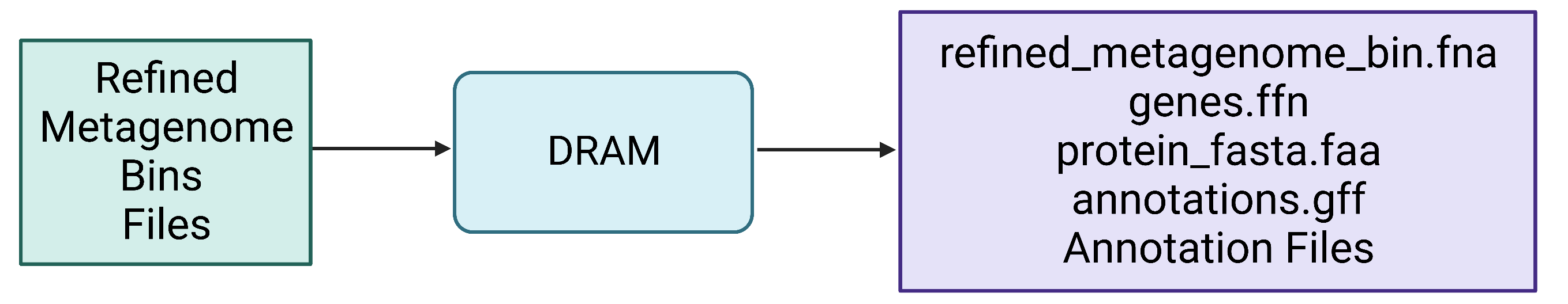
Figure 8. Refined bin FASTA files are again provided as input for DRAM, which produces a variety of output files, including gene and protein multi-FASTA files.

WARNING: Do not run DRAM! The databases it requires were too large to allow it to be installed and run on the AWS instance.

The DRAM database requires 500–700GB of storage and installing the DRAM database on a high-performance computing cluster at the University of Calgary required 32 threads and 375GB of RAM taking a day and a half to complete.

Example commands for the KGHS1-0.bin1.fa MAG:

# Change the directory back to the module5 directory.

cd /home/ubuntu/workspace/mags_workshop/module5

# Activate the conda environment.

conda activate dram_env

# Prepare the DRAM databases.

DRAM-setup.py prepare_databases –threads 32 –output_dir /path/to/dram_database

# Execute the DRAM annotation command.

DRAM.py annotate -i bin_refinement/KGHS_1-0/metawrap_50_10_bins/bin.1.fa -o refined_bins/KGHS_1-0/KGHS_1-0_bin.1/dram

# Execute the DRAM distill command.

DRAM.py distill -i refined_bins/KGHS_1-0/KGHS_1-0_bin.1/dram/annotations.tsv -o refined_bins/KGHS_1-0/KGHS_1-0_bin.1/dram/genome_summaries –trna_path refined_bins/KGHS_1-0/KGHS_1-0_bin.1/dram/trnas.tsv –rrna_path refined_bins/KGHS_1-0/KGHS_1-0_bin.1/dram/rrnas.tsv

Both steps took 26 minutes together for the KGHS_1-0_bin.1 MAG using 10 threads as it uses 10 threads as the default if you do not specify the –threads parameter.

Example output:

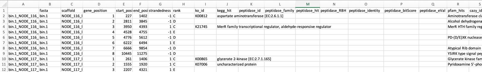
less /home/ubuntu/workspace/mags_workshop/module5/output/refined_bins/KGHS_1-0/KGHS_1-0_bin.1/dram/annotations.tsv

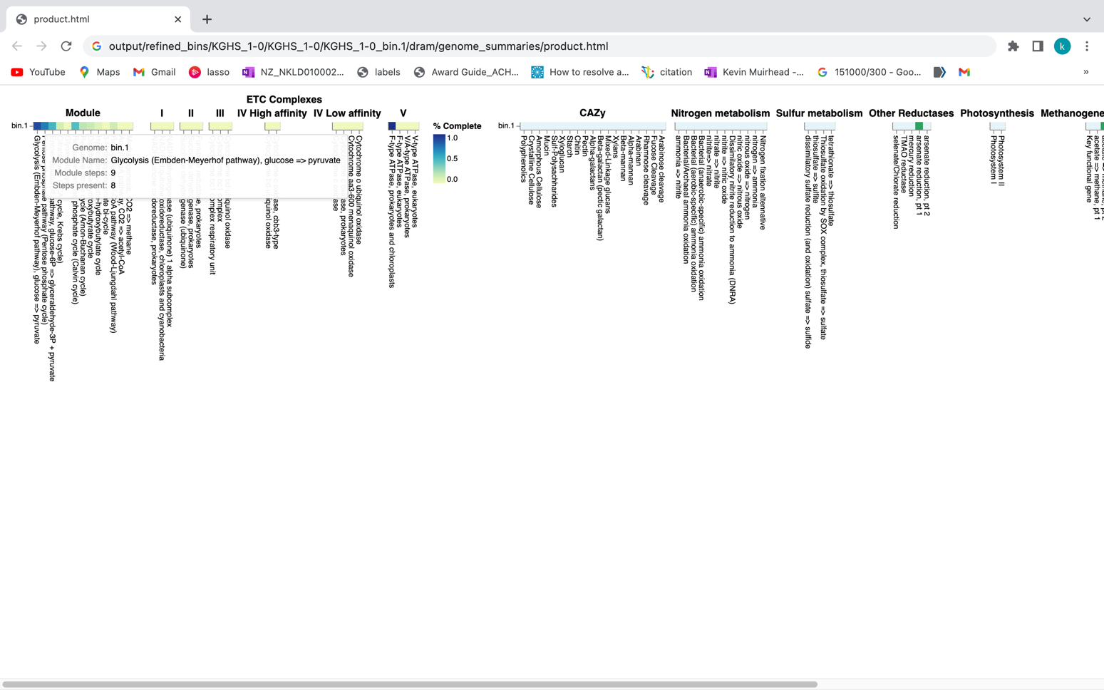
# Use a symbolic link to point to the DRAM product.html file for the KGHS_1-0_bin.1 MAG.

ln -s /home/ubuntu/workspace/mags_workshop/module5/output/refined_bins/KGHS_1-0/KGHS_1-0_bin.1/dram/genome_summaries/product.html /home/ubuntu/workspace/mags_workshop/KGHS_1-0_bin.1_product.html

# Open the KGHS_1-0_bin.1 product.html file in a browser window (i.e. chrome)

http://50.uhn-hpc.ca/mags_workshop/KGHS_1-0_bin.1_product.html

Exercises:

Question: How many pentose phosphate pathway steps are found within the KGHS_1-0_bin.1.fa MAG?

# Use a symbolic link to point to the DRAM product.html file for the KGHS_1-0_bin.3 MAG.

ln -s /home/ubuntu/workspace/mags_workshop/module5/output/refined_bins/KGHS_1-0/KGHS_1-0_bin.3/dram/genome_summaries/product.html /home/ubuntu/workspace/mags_workshop/KGHS_1-0_bin.3_product.html

# Open the KGHS_1-0_bin.3 product.html file in a browser window (i.e. chrome)

http://50.uhn-hpc.ca/mags_workshop/KGHS_1-0_bin.3_product.html

Compare the results of Prokka versus DRAM. Both use Prodigal (https://github.com/hyattpd/Prodigal) for calling open reading frames (ORFs), Barrnap (https://github.com/tseemann/barrnap) to identify 5S, 23S,16S rRNA genes. DRAM uses tRNAscan-SE (http://lowelab.ucsc.edu/tRNAscan-SE/) for t-RNA gene prediction while Prokka uses Aragorn (http://www.ansikte.se/ARAGORN/) for t-RNA gene prediction. DRAM and Prokka use a different combination of databases for annotation of protein coding genes, sometimes resulting in different gene names functional annotations.

Table 5: Overview of the programs used in the DRAM and Prokka annotation software.

Program Name	ORF caller	rRNA Prediction	t-RNA Prediction	Databases
DRAM	Prodigal	Barrnap	trnascan	UniRef90, PFAM, dbCAN, RefSeq viral, VOGDB and the MEROPS peptidase database
Prokka	Prodigal	Barrnap	ARAGORN	ISFinder, NCBI Bacterial Antimicrobial Resistance Reference Gene Database, and UniProtKB (SwissProt)

Both have similar output file types yet DRAM uses quite a few more databases giving better annotations for your MAGs. There are many other types of annotation software out there, but not all software annotate every possible type of sequence with the type of information that you might be looking for. Therefore, you may need to run other software to obtain the types of annotations that you are interested in.

Exercises:

Question: How many “hypothetical” proteins are there within the bins annotated using Prokka? How many using DRAM?

Question: How many coding sequences (CDS) did Prokka annotate versus DRAM?

Question: Do all the MAGs have a chaperonin 60 (cpn60) protein coding gene? This is an alternative marker gene to 16S rRNA that is used in many microbial ecology studies. How about the 16S rRNA gene?

Hint: The cpn60 gene in Prokka can be searched using synonyms such as GroEL and chaperonin 60 kDa. You can search ‘16S ribosomal RNA’ in Prokka, then cross reference the gene/scaffold ID in the Prokka .gff file to the one found in the DRAM annotations.tsv file.

Question: Find a GH68 levansucrase carbohydrate active enzyme (CAZyme) in the DRAM annotations.tsv file. Compare it to the annotation found in Prokka.

Hint: Search for GH68 or “levansucrase” in the DRAM annotations.tsv file. Find a scaffold ID that will link to the annotation in Prokka.

Step 3c: Annotate structural features – in this case mobile elements – of MAGs using mobileOG-db

mobileOG-db (https://github.com/clb21565/mobileOG-db)

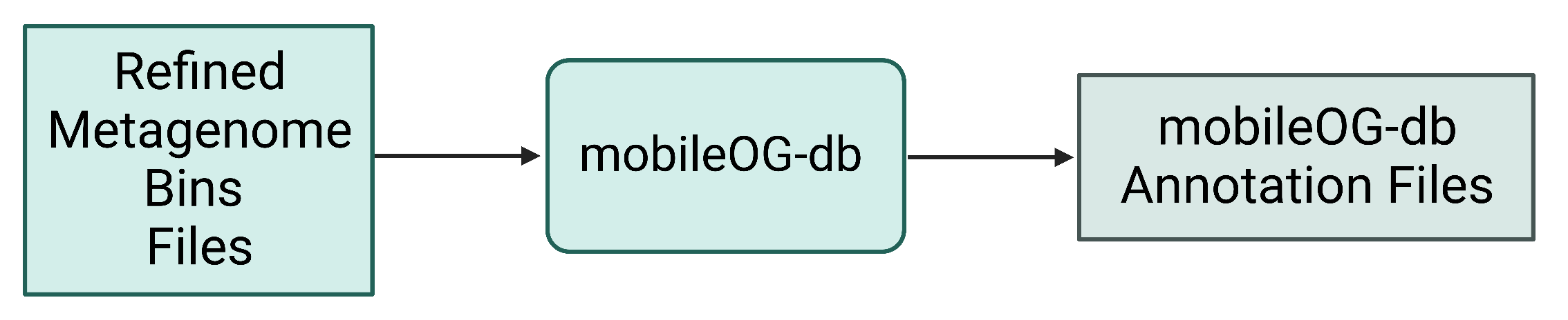
Figure 9. Refined bin FASTA files are again provided as input for mobileOG, which produces a variety of annotation files as output.

Example commands to run mobileOG-db.

# Change the directory back to the module5 directory.

cd /home/ubuntu/workspace/mags_workshop/module5

# Activate the conda environment.

conda activate mobileogdb_env

# Create the mobileogdb directory.

mkdir -p refined_bins/KGHS_1-0/KGHS_1-0_bin.1/mobileog_db

# Run diamond on the mobileOG-db.

diamond blastp -q refined_bins/KGHS_1-0/KGHS_1-0_bin.1/prokka/KGHS_1-0_bin.1.faa --db software_dir/mobileOG-db/mobileOG-db-beatrix-1.6.dmnd --outfmt 6 stitle qseqid pident bitscore slen evalue qlen sstart send qstart qend -o refined_bins/KGHS_1-0/KGHS_1-0_bin.1/mobileog_db/KGHS_1-0_bin.1.tsv --threads 14 -k 15 -e 1e-20 --query-cover 80 --id 30

# Run the mobileOG-db script for parsing the output and merging the metadata for extra information.

python software_dir/mobileOG-db/mobileOG-pl/mobileOGs-pl-kyanite.py --o refined_bins/KGHS_1-0/KGHS_1-0_bin.1/mobileog_db/annotation --i "refined_bins/KGHS_1-0/KGHS_1-0_bin.1/mobileog_db/KGHS_1-0_bin.1.tsv" -m software_dir/mobileOG-db/mobileOG-db-beatrix-1.6-All.csv

Example output:

less /home/ubuntu/workspace/mags_workshop/module5/output/refined_bins/KGHS_1-0/KGHS_1-0_bin.1/mobileog_db/annotation.mobileOG.Alignment.Out.csv

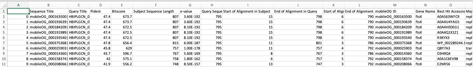
You can expect to find the following types of mobile elements;

• Insertion sequences (IS) – small pieces of DNA which move within or between genomes using their own specialized recombination systems. i.e. transposons

• Integrative genomic elements (IGEs) – mobile multigene DNA units that integrate into and excise from host bacterial genomes.

• Plasmids – small circular extrachromosomal DNA molecules that replicate and are transmitted independent from chromosomal DNA.

• Phages – bacteriophage genome that is integrated into the circular bacterial chromosome or exists as an extrachromosomal plasmid within the bacterial cell.

Open the mobileOG-db annotation.mobileOG.Alignment.Out.csv and annotation.summary.csv output files to answer the following questions.

Question: How many IS, IGE, plasmid and/or phage sequences are in the KGHS_1-0_bin.1.fa MAG? Hint: Look in the annotation.summary.csv file.

Question: Compare the annotation output of mobileOG-db to prokka. What did prokka and mobileOG-db annotate these protein sequences as? Hint: You can use the grep command to search the the annotations from mobileOG-db using the locus tag ids and grab the prokka protein fasta file.

Appendices

Appendix Section 1: Downloading SRA datasets

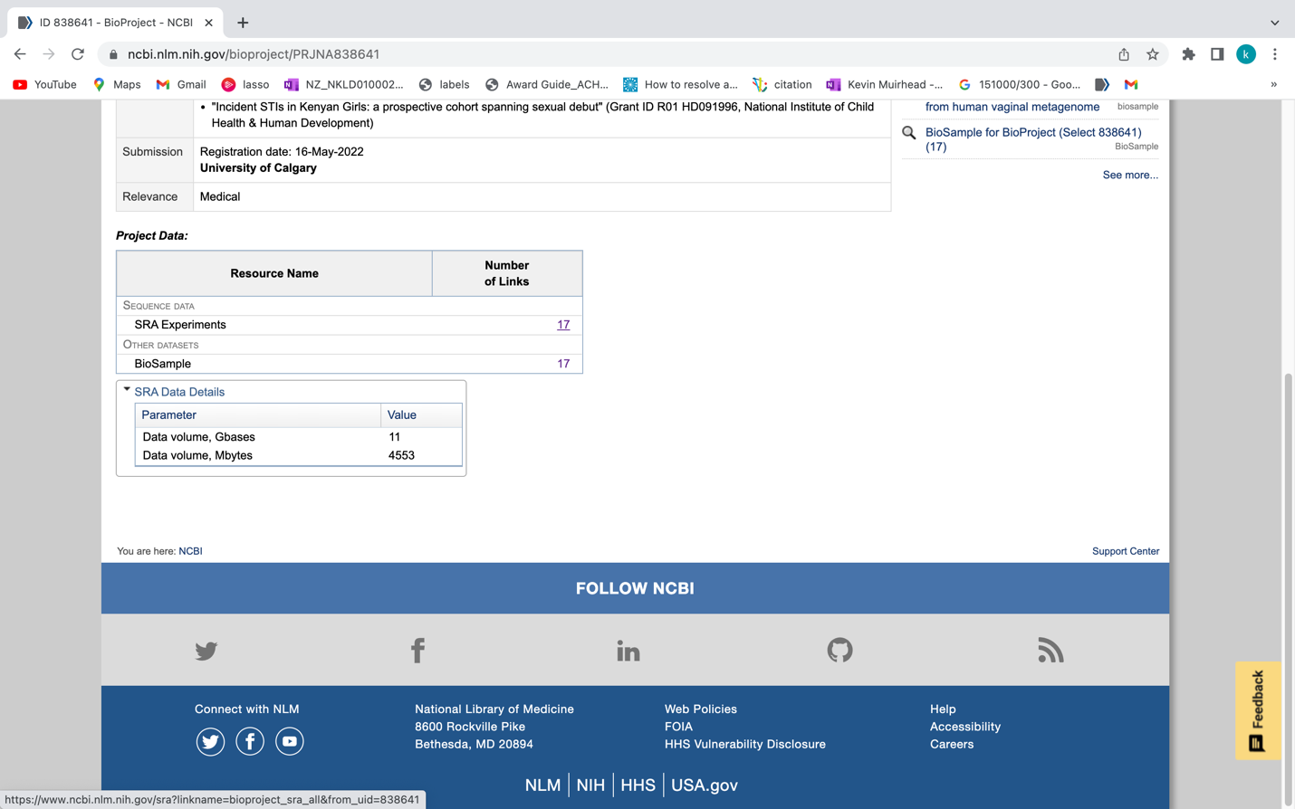
The dataset was downloaded from bioproject ID PRJNA838641 using the SraRunInfo.csv file when in the SRA list.

https://www.ncbi.nlm.nih.gov/bioproject/PRJNA838641

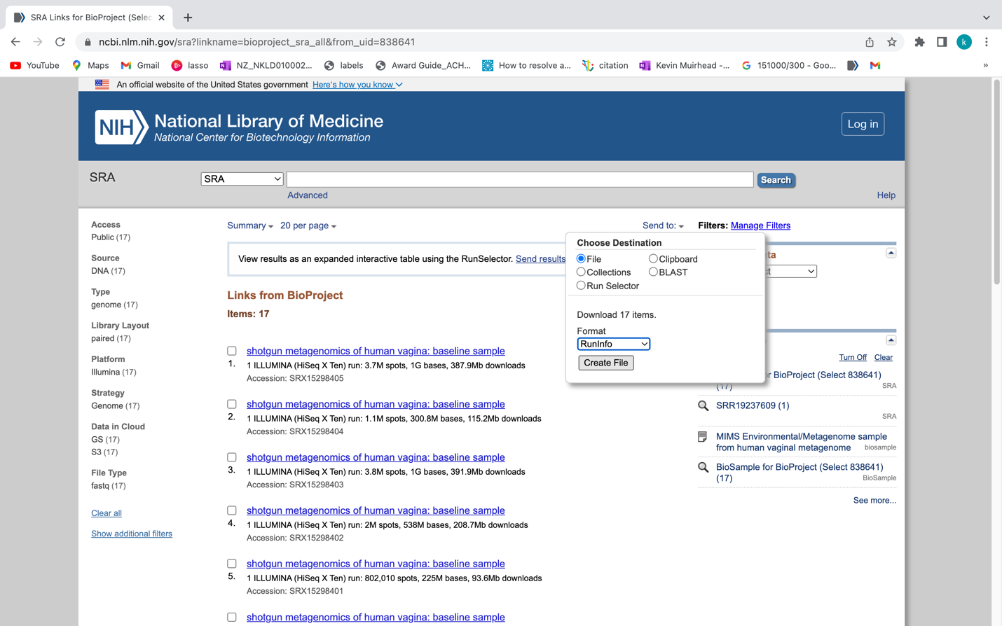
If you scroll down to the SRA Experiments section shown in the following screenshot, you will see the link labelled 17 which will take you to the SRA experiment page. For your convenience we have provided the following link (https://www.ncbi.nlm.nih.gov/sra?linkname=bioproject_sra_all&from_uid=838641)

Once you are at the following page you can click on the “Send to:” drop down menu and select “File”, then the Format drop down menu and select “RunInfo” and click “Create File”. This will download a file called “SraRunInfo.csv” which lists each SRA entry for the KGHS Pilot Dataset with each having an SRA Run ID and a sample name in the file that we can use to download each shotgun metagenome paired end read set using the fasterq-dump program within the NCBI SRA toolkit.

We can then use the “SraRunInfo.csv” file to download each sample using fasterq-dump if we wanted. An example shell script “download_sra_dataset.sh” has been provided in github.com so that you can use it to download public shotgun metagenomics datasets from NCBI to use in your research. You can do this on your own time if you are interested in incorporating public NCBI SRA datasets to your research using a NBCI BioProject ID from a paper related to your work.

For the purpose of this tutorial we have selected a subset of the data with four samples so that you can follow along before applying what you have learned to larger public datasets. We used the shell script “download_sra_subsampled_dataset.sh” to download the four samples we selected. An example of the fasterq-dump command is shown below. The command is set to use 4 threads to make the process a bit faster. The output file name is specified as the sample name KGHS_8-0 and the output directory is specified cleaned_fastq_files. The –split-files option converts the SRA to fastq files automatically, and splits the reads into read 1 and read 2 files.

Example command:

fasterq-dump –threads 4 –outfile KGHS_1-0 –outdir cleaned_fastq_files –split-files SRR19237623

Appendix 2: Shell scripts and slurm job array submission scripts.

We made the shell scripts available as examples of how to run these scripts in a more high-throughput fashion. If you have a high-performance computing (HPC) cluster running SLURM to submit jobs we supplied shell scripts and job array sbatch scripts for your use following all four samples detailed in this tutorial. If you do not have access to a HPC cluster using SLURM we have also provided the same scripts using a for loop to iterate over the sample and binned MAGs for each sample depending on the command instead of job arrays for your convenience. Please go to the bioinformatics.ca github repository to download these scripts for your use. Follow the instructions there for how to install the conda environments, databases and running the scripts.

https://github.com/bioinformaticsdotca/MIC_2023/blob/main/module5/scripts

Appendix 3: Extra annotation programs and examples.

Alternate function annotation tool: eggnog-mapper.

eggnog-mapper (https://github.com/eggnogdb/eggnog-mapper)

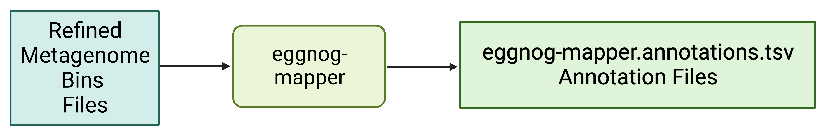
The eggnog-mapper program annotates a protein.fasta file using databases download using the download_eggnog_data.py (https://github.com/eggnogdb/eggnog-mapper) script.

Example command:

# Change the directory back to the module5 directory.

cd /home/ubuntu/workspace/mags_workshop/module5

# Activate the eggnog_mapper conda environment.

conda activate eggnog_mapper_env

# Create the eggnog_mapper directory.

mkdir -p refined_bins/KGHS_1-0/KGHS_1-0_bin.1/eggnog_mapper

# Run the eggnog-mapper annotation command using the prokka protein fasta file as input.

python path/to/software_dir/eggnog-mapper/emapper.py -i refined_bins/KGHS_1-0/KGHS_1-0_bin.1/prokka/KGHS_1-0_bin.1.faa –itype proteins –cpu 14 –data_dir /path/to/eggnog-mapper/data –output refined_bins/KGHS_1-0/KGHS_1-0_bin.1/eggnog_mapper/KGHS_1-0_bin.1

Example output:

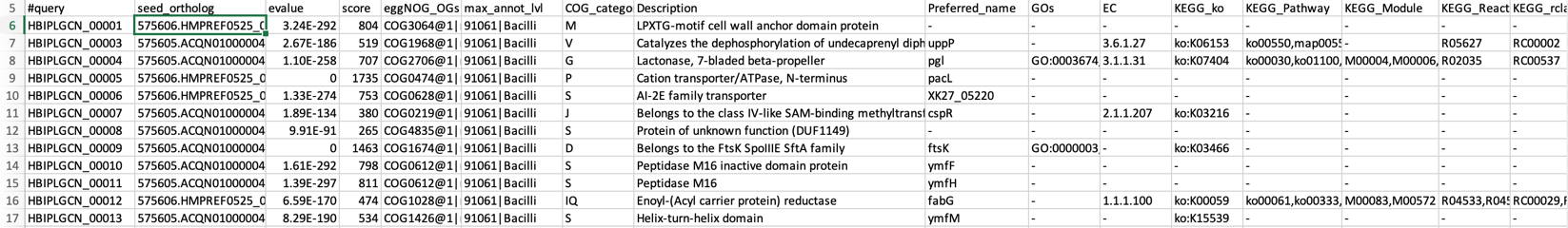
less /home/ubuntu/workspace/mags_workshop/module5/output/refined_bins/KGHS_1-0/KGHS_1-0_bin.1/eggnog_mapper/KGHS_1-0_bin.1.emapper.annotations

#query – The query name

seed_ortholog - The seed ortholog ID

evalue – The seed ortholog e-value

score - The seed ortholog bit score

eggNOG_OGs - A comma-separated, clade depth-sorted (broadest to narrowest), list of Orthologous Groups (OGs) identified for this query. Note that each OG is represented in the following format: OG@tax_id|tax_name

max_annot_lvl - tax_id|tax_name of the level of widest OG used to retrieve orthologs for annotations.

COG_category - COG category of the narrowest OG with a valid assignment.

Description - Description of the narrowest OG with a valid assignment.

Preferred_name – The preferred name of the protein sequence.

GOs – Gene Ontology IDs

EC – Enzyme class number

KEGG_ko – KEGG ko ID

KEGG_Pathway – KEGG pathway ID

KEGG_Module – KEGG module ID

KEGG_Reaction – KEGG reaction ID

KEGG_rclass – KEGG rclass information.

BRITE – KEGG BRITE ID

KEGG_TC – KEGG TC

CAZy – The carbohydrate active enzyme annotation (cazy.org)

BiGG_Reaction – The Biochemically, Genetically and Genomically structured genome-scale metabolic network reconstructions.

PFAMs – PFAM IDs

Question: How does eggnog-mapper compare to the results of DRAM? Did we annotate the same number of CDS sequences? Are the annotations named the same? Hint: Since we are starting with the prokka protein fasta file .faa the sequence IDs will be different but using the annotations you can figure out what scaffold they came from and the start and end positions of the open reading frames.

Step 4: Annotate MAGs using dbCAN

run_dbCAN4 (https://github.com/linnabrown/run_dbcan)

The run_dbcan software annotates a protein fasta file with carbohydrate active enzymes[13]. run_dbcan4 is a new version that uses eCAMI HMM models to obtain the enzyme class number (EC#) to predict the substrate a CAZyme.

# Change the directory back to the module5 directory.

cd /home/ubuntu/workspace/mags_workshop/module5

# Activate the run_dbcan conda environment.

conda activate run_dbcan_env

# Create the eggnog_mapper directory.

mkdir -p refined_bins/KGHS_1-0/KGHS_1-0_bin.1/dbcan

# Run the run_dbcan command.

run_dbcan refined_bins/KGHS_1-0/KGHS_1-0_bin.1/prokka/KGHS_1-0_bin.1.faa protein –db_dir /home/ubuntu/workspace/mags_workshop/module5/software_dir/run_dbcan_database –dia_cpu 14 –hmm_cpu 14 –dbcan_thread 14 –out_dir refined_bins/KGHS_1-0/KGHS_1-0_bin.1/dbcan

less /home/ubuntu/workspace/mags_workshop/module5/output/refined_bins/KGHS_1-0/KGHS_1-0_bin.1/dbcan/overview.txt

Example output from overview.txt. Open the KGHS_1-0_bin.1 overview.txt file using the less command. You will see the following columns. One row for each CAZyme classified.

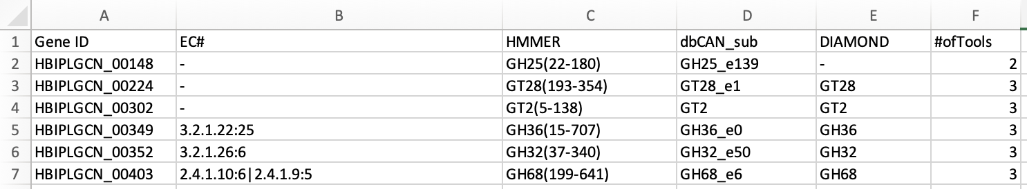
Gene ID – The prokka locus tag

EC# - The enzyme class number (if present)

HMMER – The results from the dbcan HMM model.

dbCAN_sub – The dbcan substrate prediction using the eCAMI kmer HMM model. Reports the CAZyme family and the substrate ID.

DIAMOND – The DIAMOND results from the dbcan protein fasta database.

#ofTools - The number of tools that annotated this Gene ID

Excercises:

Question: How does the CAZy results in eggnog-mapper compare to the results given by run_dbCAN4?

Question: How does the CAZy results in DRAM compare to the results of run_dbCAN4?

Question: How do you search for the details of a CAZyme family on the Carbohydrate-Active enZYmes Database site (http://www.cazy.org/)? Hint: Use the search bar with the “Family” dropdown box.

References

1. Prjibelski, A., et al., Using SPAdes De Novo Assembler. Current Protocols in Bioinformatics, 2020. 70(1): p. e102.

2. Gurevich, A., et al., QUAST: quality assessment tool for genome assemblies. Bioinformatics, 2013. 29(8): p. 1072-1075.

3. Peng, Y., et al., IDBA-UD: a de novo assembler for single-cell and metagenomic sequencing data with highly uneven depth. Bioinformatics,

1. 28(11): p. 1420-1428.

4. Li, D., et al., MEGAHIT: an ultra-fast single-node solution for large and complex metagenomics assembly via succinct de Bruijn graph. Bioinformatics, 2015. 31(10): p. 1674-1676.

5. Shen, W., et al., SeqKit: A Cross-Platform and Ultrafast Toolkit for FASTA/Q File Manipulation. PLOS ONE, 2016. 11(10): p. e0163962.

6. Kang, D.D., et al., MetaBAT 2: an adaptive binning algorithm for robust and efficient genome reconstruction from metagenome assemblies. PeerJ, 2019. 7: p. e7359.

7. Wu, Y.-W., B.A. Simmons, and S.W. Singer, MaxBin 2.0: an automated binning algorithm to recover genomes from multiple metagenomic datasets. Bioinformatics, 2015. 32(4): p. 605-607.

8. Li, H., Aligning sequence reads, clone sequences and assembly contigs with BWA-MEM. arXiv: Genomics, 2013.

9. Li, H., et al., The Sequence Alignment/Map format and SAMtools. Bioinformatics, 2009. 25(16): p. 2078-2079.

10. Parks, D.H., et al., CheckM: assessing the quality of microbial genomes recovered from isolates, single cells, and metagenomes. Genome Res, 2015. 25(7): p. 1043-55.

11. Song, W.Z. and T. Thomas, Binning_refiner: improving genome bins through the combination of different binning programs. Bioinformatics,

1. 33(12): p. 1873-1875.

12. Chaumeil, P.-A., et al., GTDB-Tk: a toolkit to classify genomes with the Genome Taxonomy Database. Bioinformatics, 2019. 36(6): p. 1925-1927.

13. Zhang, H., et al., dbCAN2: a meta server for automated carbohydrate-active enzyme annotation. Nucleic Acids Research, 2018. 46(W1): p. W95-W101.