Informatics and Statistics for Metabolomics 2018 Module 2 Lab
Module 2 Lab: Metabolite Identification and Annotation
In this lab, you will perform metabolite ID and/or quantification using NMR data and Bayesil; GC-MS data and GC-AutoFit; and LC-MS data and XCMS.
NMR
Example Data
The sample data is from a study comparing healthy controls to endometrial cancer cases in females. The sample type is human serum. There are 40 samples total, 20 controls and 20 cases. The study population are female adults over the age of 18 with a mean age of 59.2 +/- 12.7 years for the controls and 59.1 +/- 12.8 years for the cases.
General Instructions
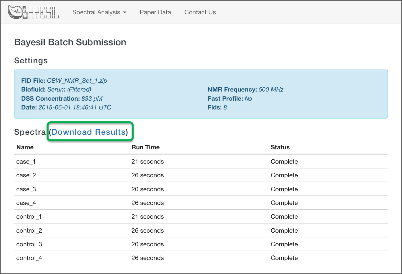
We will be using Bayesil for analysis of the NMR data. The NMR data files are available here. The .zip folder contains 5 data sets. Upload one of the datesets into Bayesil and run the server. Save the results as an Excel file. Examine the results by eye to find interesting differences. Use HMDB to learn about the interesting metabolites.
Bayesil
Bayesil is a web-based tool for automated NMR spectral profiling that is very accurate (95%) and which uses probabilistic graphical models (PGM). It fits shift and peak intensity similar to the way humans perform fitting and pattern finding. Bayesil requires priop knowledge of probable biofluid composition. It has fully automated phasing, referencing, water removal, baseline correction, identification, and quantification.
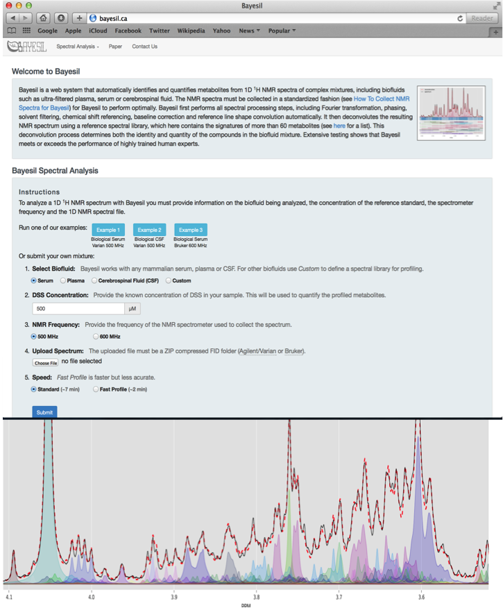
Bayesil Example Settings
| Biofluid | Serum |
| Chemical Shift (CS) Reference | DSS |
| CS Reference Concentration | 833 um |
| NMR Frequency | 500 MHz |
| Compressed FIDS | One of: CBW_NMR_Set_1.zip, CBW_NMR_Set_2.zip, CBW_NMR_Set_3.zip, CBW_NMR_Set_4.zip, CBW_NMR_Set_5.zip |
| Speed | Standard |
Bayesil Batch Results
Bayesil Spectrum Results

GC-MS
Example Data
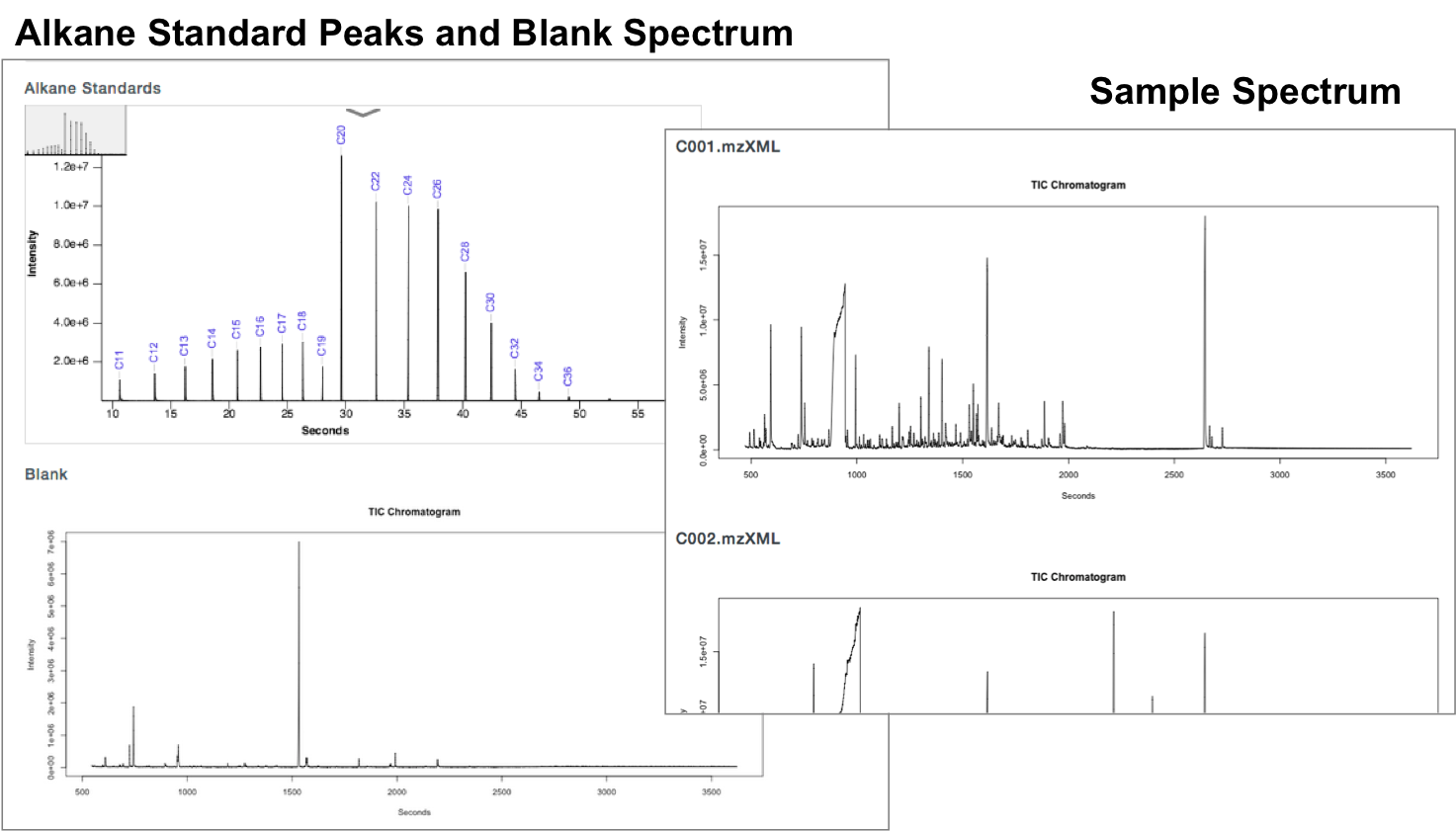
The sample data is from a study comparing 20 individuals with Eosinophilic Esophagitis (EoE) with 20 healthy controls, ages 3-13. The sample type is urine with an internal standard control of cholesterol. The Jul0914 file has 1 Alkane standard, 1 blank sample, and 20 samples. The Jul1114 file also has 1 Alkane standard, 1 blank sample, and 20 samples.
General Instructions
We will be using the GC-AutoFit website for analysis of our data. The data 2 data files can be found here and here. Upload the files to GC-AutoFit adn run the server. Save the results as an Excel file. Examine the results by eye to find interesting differences. Use HMDB to learn about the interesting metabolites.
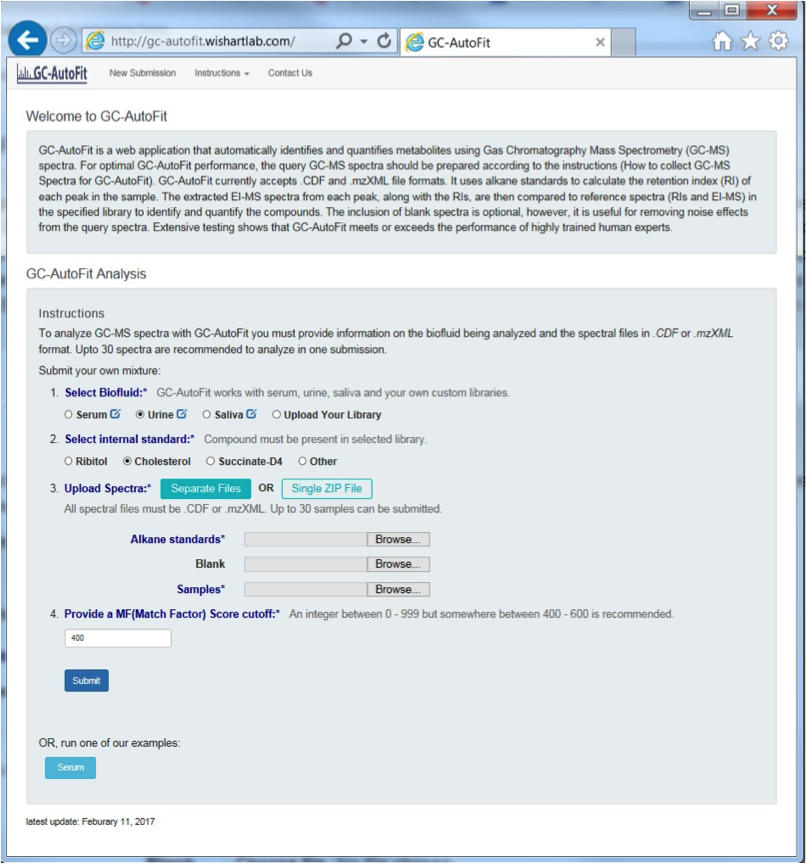
GC-AutoFit (Automated GC-MS)
GC-AutoFit websitet requires 3 spectra (sample, blank, and alkane standard). It performs auto-alignment, peak ID, peak integration, and concentration calculation. It accepts NetCDF and mzXML files. It takes 60 seconds per spectrum with 40-115 compounds ID’d at 96% accuracy. It is optimized for blood, urine, saliva, and cerbral spinal fluid. It still requires careful sample preparation and derivatization.
Preparing GC-MS Spectral Files
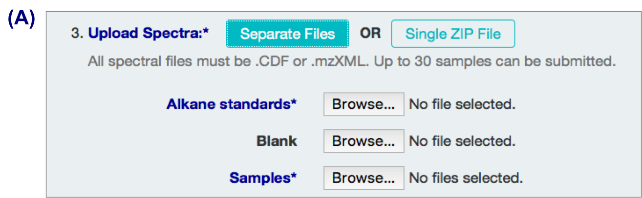
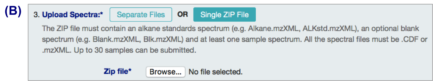
3 types of input files:
- alkane standard file (required; eg Alkane.mzXML, ALKstd.mzXML)
- a blank sample file (optional but recommended; eg Blank.mzXML, Blk.mzXML)
- Sample files (required)
Your files might require format conversion. Files are expected to be CDF or mzXML. “.D” format can be converted to “.CDF” or “.mzXML” format with conversion software such as ChemStation or ProteoWizard.
Uploading GC-MS Spectral Files
A. Individual files
B. .zip files
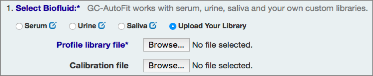
Select Sample Type and Library
You can either select an internal library (serum, urine/organic acids, saliva, etc) or a user library.
Set an internal standard for quantification:
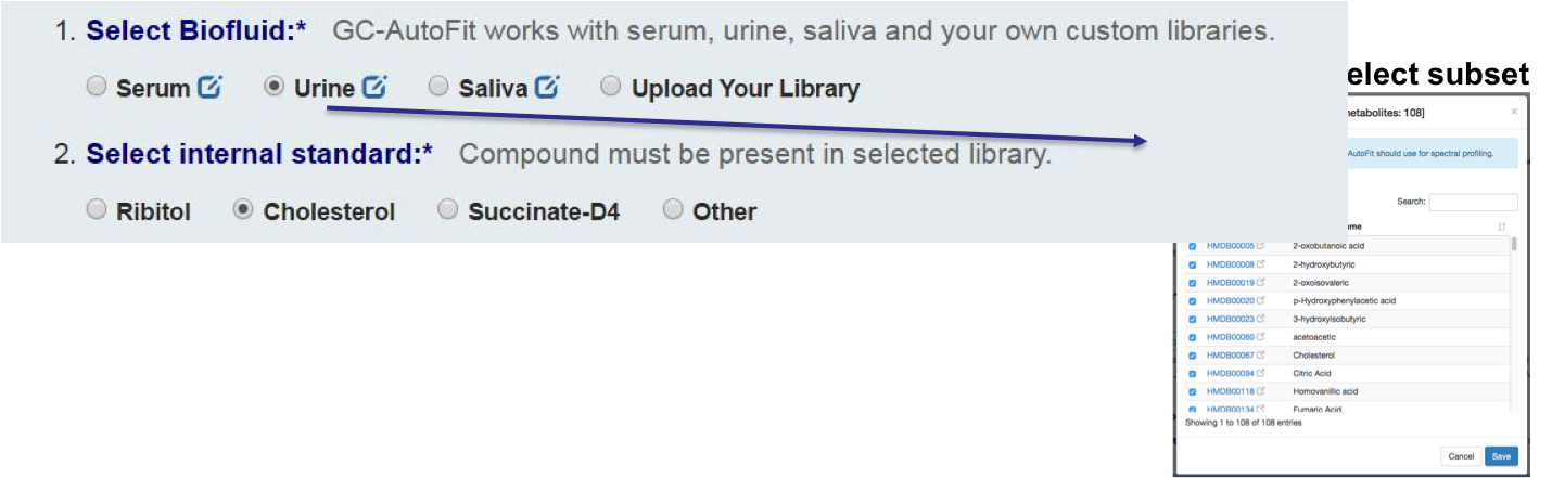
or
Check Alkane Standard and Each Sample Spectrum
Profiling and Quantification
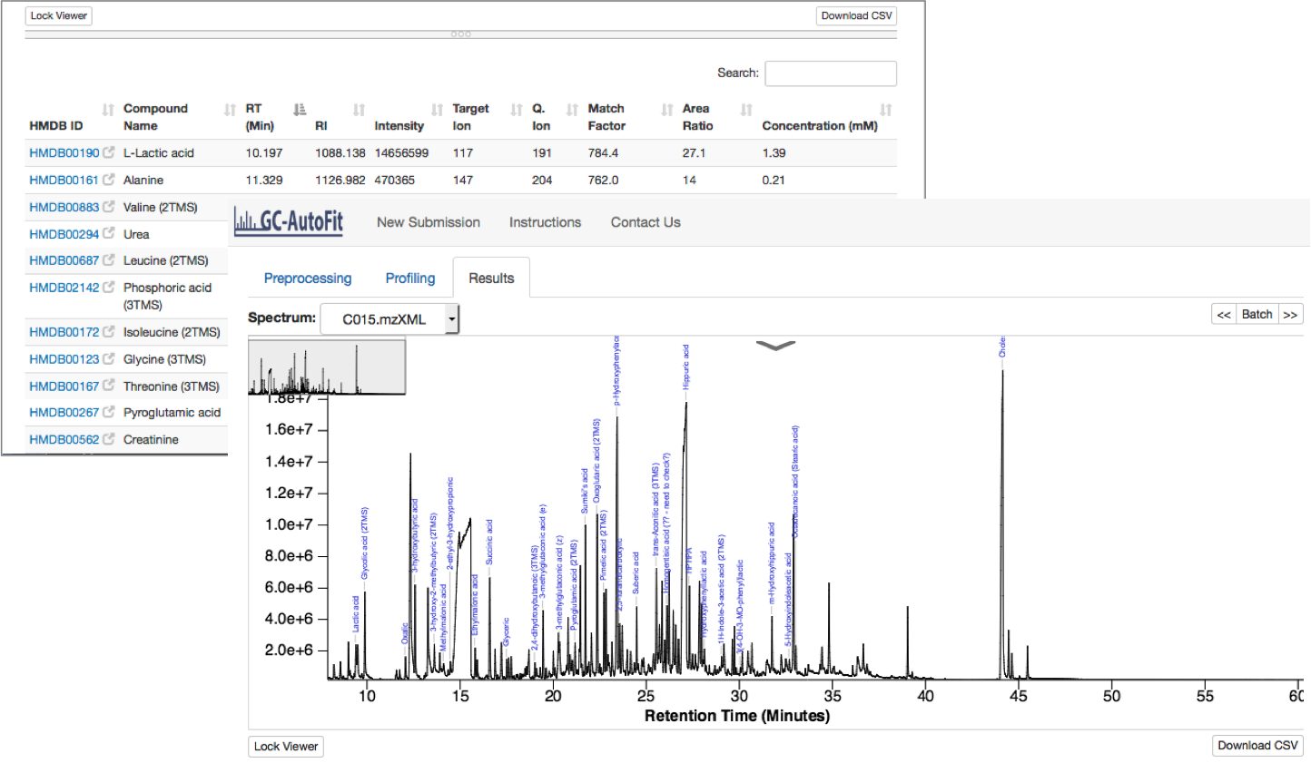
Final Results
Results are reported as a table (csv format) for each sample and merged concentrations for all samples.

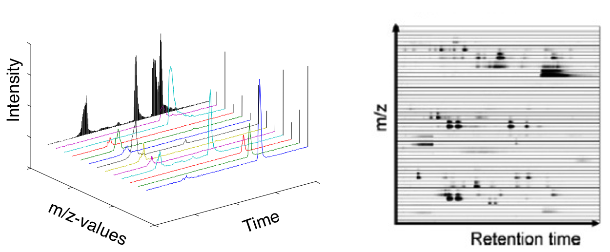
LC-MS
Do this section only if you are comfortable using R
You will need R with the XCMS packages installed. You can optionally have ProteoWizard installed. The data files are provided as raw files or mzXML converted files.
Example Data
This dataset was acquired using RP-HPLC-MS (Orbitrap) in positive ionization mode (m/z range 90-800 over 25min). The 30 samples are a subset of a larger study, and include urine samples from people with chronic kidney disease (CKD) stage 3b to stage 5, and controls (a few have CKD stage 2). The Metadata has more information.
Raw datasets (raw.zip files)
Converted datasets (mzxml.zip files)
XCMS using R (results files)
XCMS online (results files)
Cleaned Diffreport
Normalized Results
Unnormalized Results
XCMS Installation
# use biocLite to install a Biocondcutor package
source("http://bioconductor.org/biocLite.R")
# Install the xcms package # make sure that the R folder is not read only; define .libPaths
biocLite("xcms")
# Install multtest package for diffreport function
biocLite("multtest")
# check that all packages are in place
loadedNameSpaces() # Load the XCMS package
library(xcms)
R Commands Overview
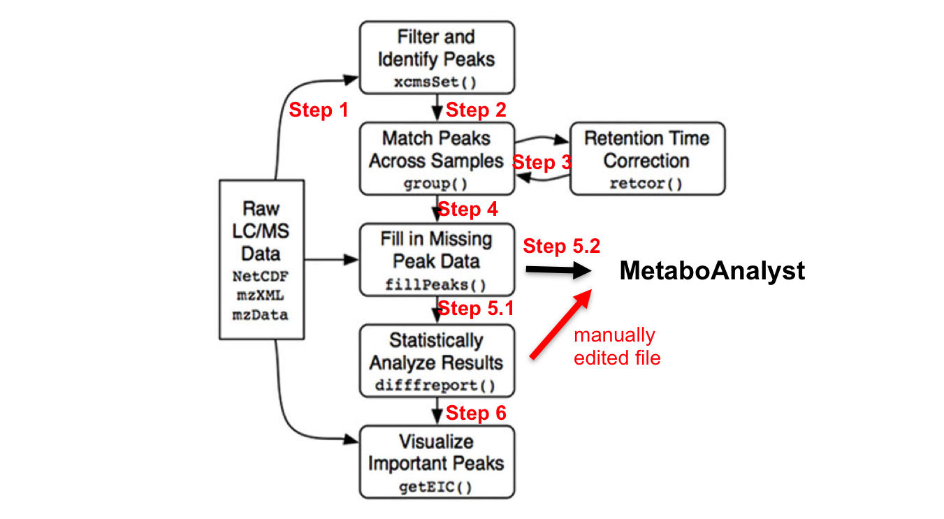
library(xcms)
# in  – parameter sets further detailed in each step; # some steps are destructive, hence name is changed to allow re-processing the previous step if necessary.
mzxmlfiles <- list.files(full.names=TRUE, recursive= TRUE) # input files (step 1)
xset <- xcmsSet (mzxmlfiles, )  # peak picking (step 2)
xset1 <- group (xset)    # peak grouping and matching between samples (step 3.1)
xset2 <- retcor (xset1, )  # retention time correction. (step 3.2)
xset2 <- group (xset2, )  # re-alignment due to previous step (step 3.3)
xset3 <- fillPeaks (xset2)  # filling in missing peak data (step 4) # optional median-fold normalization step; requires obtaining the function code first
normalData <- cbind(groups(xset3), normalize.medFC(groupval(xset3, "medret", "into")) )
write.csv(normalData, file="medFoldNorm.csv")
dat <- groupval (xset3, "medret", "into")  # get peak intensity matrix (step 5)
dat2 <- rbind (group = as.character(phenoData(xset3)$class), dat)  # add group label
write.csv (dat, file=‘PeakTable.csv’)  # save the data to CSV file
dr <- diffreport (xset3, ) # (step 5.1)
write.csv (dr, file="diffreport.csv")
Prepare Inptut (Step 1)
XCMS package file compatibility:
- mzXML, mzData and NetCDF (AIA/ANDI format).
Software for most instruments can export to NetCDF and also to mzxml, a common file format. There are free tools for data conversion.
XCMS online file compatibility:
- AB Sciex .wiff
- Agilent .d (.D need to be exported from chemstation as .AIA)
- Bruker .d, YEP, BAF, FID
- Thermo .raw
- Waters. raw
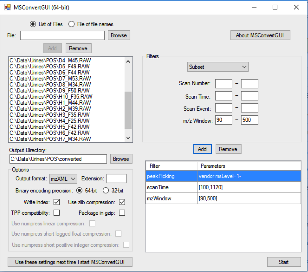
ProteoWizard “MSConvert” is a free file conversion tool:
Put all .mzXML files in a folder named “DataSet” under your current working directory. Place files from each experimental class under a separate sub-folder.
# set working directory to the folder with the dataset. You can copy the path      # from the location in the properties of the folder, but replace \ by /
setwd (“C:/..”))
getwd ()   # confirm
# create path to all the input files. can use parameter pattern=".mzXML“.
# recursive= TRUE: include all sub directories (for the experimental classes)
mzxmlfiles <- list.files(full.names=TRUE, recursive= TRUE)
# view the file list within the working directory
mzxmlfiles
Peak Detection (step 2)
XCMS parameters depend on the type of LC-MS instrument, method, ionization mode, performance and more. requires further learning and experimenting.
# CAN TAKE A FEW MINUTES OR LONGER, DEPENDING ON THE COMPUTER.
# Calling xcmsSet function to process all mzxmlfiles using parameters set 1
# order of parameters is not important; all time parameters are in seconds!
xset <- xcmsSet (mzxmlfiles, method="centWave", ppm=1.5, polarity="positive", peakwidth= c(10,60),snthresh= 20,prefilter= c(7,20000), integrate=1,mzdiff=0.005)
xset   # get a short report on the results
Some important parameters in parameter set 1:
method = ‘centWave: use wavelet algorithm for peak detection, suitable for high resolution spectra;
ppm: max deviation between consecutive scans;
polarity: positive or negative ionization mode;
scanrange = c(lower, upper): scan part of the spectra (done in ProteoWizard to reduce file size);
snthresh = x: minimum signal-to-noise ratio;
prefilter = c(how many peaks, with peak intensity);
integrate= 1 or 2 (2 more accurate but suffers from more noise);
mzdiff = x: in coeluting peaks, what is the minimum difference in m/z to be considered different peaks (instrument dependant).
Peak Alignment adn Retention Time Correction (step 3.1 - 3.3)
Step 3.1: Matching peaks across samples
Step 3.2: Using the peak groups to correct retention drift
Step 3.3 Re-do the peak alignment (2nd time, reducing the group)
Can be performed iteratively until no further change
# peak grouping and matching between samples (step 3.1)
xset1 <- group (xset)
# retention time correction (step 3.2) using parameters set 2
xset2 <- retcor (xset1, method="obiwarp", plottype="deviation")
# re-alignment (step 3.3) using parameters set 3
# xset2 <- group (xset2, bw=15, minfrac=0.5, mzwid=0.015, minsamp=8)
“retcor” parameter set 2: method = #algorithm for rt correction; plottype= # image of the procedure.
“group” parameter set 3: bw= #retention time deviation (in seconds) between the peaks in a group;
minfrac = #minimum fraction of samples in one class required to have the peak to define it as a group;
minsamp= #same, but total number of samples;
mzwid= # deviation in m/z between samples, allowed in one grouped peak.
Retention Time Deviation
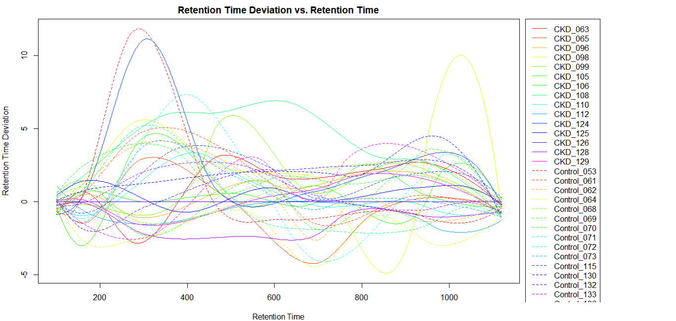
- If there are less than 20 samples, it is possible to visually identify the chromatographic outlier. It can then be replaced, or its original chromatogram fixed (decision depends on reasons – technical; biological; requires statistical considerations).
- In XCMS package it is possible to choose the sample used for alignment (in XCMS online it is the sample with the most features)
- If the deviation is in a non-relevant retention area, then its impact is low.
Filling in Missing Peaks (Step 4)
- A significant number of potential peaks can be missed during peak detection
- Missing values are problematic for robust statistical analysis
- We now have a better idea about where to expect real peaks and their boundaries
- Re-scan the raw spectra and integrate peaks in the regions of the missing peaks
# fill in missing peak data (step 4)
xset3 <- fillPeaks (xset2)
Some warnings may show up when the expected peak (as indicated by many other files) are beyond the “end” of the file. There is no raw data available for fillPeaks(). These warnings can be ignored.
Preliminary Statistical Analysis with XCMS (Step 5.1)
- XCMS ‘diffreport’ is a summary report which includes feature values of all samples as well as t-statistics.
- Multivariate analysis and visualization can be performed using MetaboAnalyst, allowing more flexible and controlled analysis
# create diffreport from the processed data or median-fold normalized data (step 5)
# need to declare the two experimental classes
# might have a few duplicate row names
dr <- diffreport (xset3, "Control", "CKD")
# export the diffreport to a file, in the working directory (by default)
write.csv(dr, file="diffreport.csv")
diffreport parameter set 4: class names (correspond with folder names in working directory);
eicwidth= x : width (in seconds) of extracted ion chromatogram plots;
metlin= 0 : (no column for metlin m/z search), or 0.001 (search metlin for ±0.001Da).
File Preparation for Statistical Analysis with MetaboAnalyst (step 5.2)
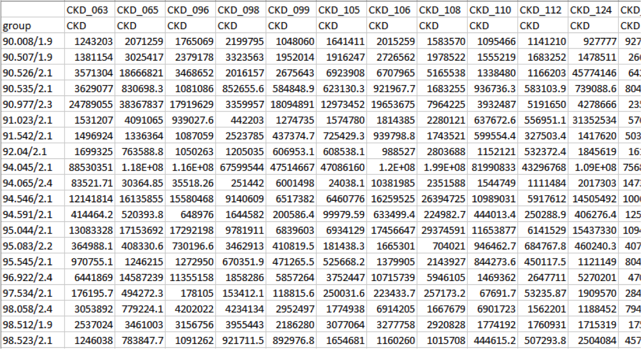
The general format required by MetaboAnalyst and most other statistical tools is a data matrix:
- Features (combination of retention time and m/z) in rows;
- Samples, in columns;
- Experimental class labels;
dat <- groupval(xset3, "medret", "into")  # get peak intensity (area) matrix
# add class labels:
dat2 <- rbind(class= as.character(phenoData(xset3)$class), dat)
# create unique feature name and retention time in minutes.
rownames(dat2) <- c("group", paste(round(groups(xset3)[,"mzmed"], 3),
+ round(groups(xset3)[,"rtmed"]/60, 1), sep="/"))
# save the data to CSV file in the WD:
write.csv(dat2, file= "PeakTable.csv")
Peak Area Table
Peaks are identified by “m/z retention time”. The file can be directly uploaded to MetaboAnalyst but further file manipulations are recommended prior to statistical analysis.
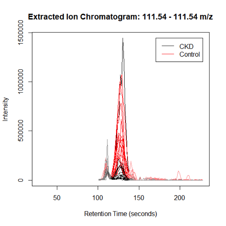
Visualizing Peaks (step 6)
When significant peaks are identified, it is critical to visualize these peaks to assess quality.
This is done using the Extracted ion chromatogram (EIC), and can also be conducted in XCMS online.
Since the XCMS results depend on the quality of data processing, it is highly recommended to examine the original chromatographic peaks and spectra in the vendor software
gt <- groups (xset3)  # get peak count table
gt [1:3, ]    # check out the first three records
# select peaks that appear at least in 25 samples, between rt of 120 - 220 seconds
groupidx1 <- which(gt[,"rtmed"] > 120 & gt[,"rtmed"] < 220 & gt[,"npeaks"] == 25)
eiccor <- getEIC(xset3, groupidx = groupidx1)
# plot the EIC for the first feature in the selected range:
plot (eiccor, xset3, groupidx = 1)