Genome-scale Multilocus Sequence Typing CBW Tutorial

Dillon Barker - 1 May, 2017

Learning Objectives

Students will learn to:

• Use chewBBACA and R to create a prototype core genome multilocus sequence typing systems
• Identify some common pitfalls in cgMLST design
• Analyze a dataset using genome-scale MLST and PHYLOViZ
• Compare typing method partitioning using the Adjusted Wallace Coefficient

Due to constraints regarding the length of time that chewBBACA takes to complete its analysis versus the length of this tutorial, many of the the steps will be given to you “kitchen show style”, i.e. I have already generated the results for several steps. The instructions for running chewBBACA are given, but there is no need to runthem here (though feel free to do so at home!). However, the later steps involving analysis in R and Phyloviz will be hands-on.

Dataset

The genome sequence dataset we’ll be analyzing here is taken from this study of a Vibrio cholerae outbreak in Haiti, which was determined to have had an epidemiologic relationship with Nepalese UN peacekeepers in the aftermath of the 2010 Haitian earthquake.

Katz LS, Petkau A, Beaulaurier J, Tyler S, Antonova ES, Turnsek MA, Guo Y, 
Wang S, Paxinos EE, Orata F, Gladney LM, Stroika S, Folster JP, Rowe L,
Freeman MM, Knox N, Frace M, Boncy J, Graham M, Hammer BK, Boucher Y, Bashir A,
Hanage WP, Van Domselaar G, Tarr CL. 2013. Evolutionary dynamics of Vibrio
cholerae O1 following a single-source introduction to Haiti.
mBio 4(4):e00398-13. doi:10.1128/mBio.00398-13. 

First, retrieve the pre-cooked chewBBACA data by running the following commands. Run the following commands in bash (the terminal on your ubuntu instance).

cd ~/workspace
wget -O cgmlst.zip https://github.com/dorbarker/CBW/archive/master.zip
unzip cgmlst.zip

ls  # you should see a directory called "CBW-master"; if not, ask a TA for help

Running chewBBACA

Calculate the pangenome

As mentioned above, there’s no need to run these right now.

ls haiti-assemblies/*.fasta > haiti-assemblies.txt

python chewBBACA/createscheme/PPanGen.py \
	-i haiti-assemblies.txt \
	-o haiti \
	--cpus 8  # or as appropriate

Call Alleles

ls haiti/*.fasta > haiti-genes.txt

python chewBBACA/allelecall/BBACA.py \
	-i haiti-assemblies.txt \
	-g haiti-genes.txt \
	-o haiti \
	--cpus 8

Filter Results

We can analyze chewBBACA’s output using R. chewBBACA will assign an allele number if can find the locus, otherwise it will return one of the following codes instead:

• EXC
  • alleles that have 100% identity
• INF
  • inferred allele with prodigal
• LNF
  • number of loci not found
• PLOT
  • loci on edges of contigs
• NIPL
  • non-informatics paralogous loci
• ALM
  • alleles 20% larger than reference locus size
• ASM
  • alleles 20% smaller than reference locus size

library(ggplot2)

setwd('~/workspace')

# First let's look at a summary of different kinds of incomplete
# calls (missing, truncated, etc) that chewBACCA assigned

stats <- read.table('~/workspace/CBW-master/haiti/chewbbaca_results/results_statistics.tsv',
			sep = '\t', header = TRUE, stringsAsFactors = FALSE, row.names = 1)

View(stats)

# now load the tab-delimited table of allele calls
calls <- read.table('~/workspace/CBW-master/haiti/chewbbaca_results/results_alleles.tsv',
			sep = '\t', header = TRUE, row.names = 1,
			stringsAsFactors = FALSE)

# convert data.frame values to integers
# this will coerce non-integer values, e.g. "LNF" to NA

allele_calls_only <- function(col) suppressWarnings(as.integer(col))

calls[] <- lapply(calls, allele_calls_only)


# We can use this function to count how many genes had an assignable allele
#
# It works by first getting a vector of all non-NA values,
# and returning its length

found_allele <- function(genes) length(na.omit(genes))

# Calculate the number of present genes per genome
genomewise_presence <- apply(calls, 1, found_allele)

# Get a six-number summary of genomewise_presence
summary(genomewise_presence)

qplot(genomewise_presence, geom = 'histogram', binwidth = 10)

Hmm. Some of the genomes have far fewer genes present than the median. This likely indicates that the sequence does not represent the species its supposed to, or the sequence is of the correct species and merely of poor quality. In either case, we should remove them from the analysis before continuing.

# We'll remove the outliers - here that happens to be roughly 
# the bottom quartile. In other datasets, this value is likely to be
# different.

remove_idx <- which(genomewise_presence < 3206)
genomes_to_remove <- rownames(calls)[remove_idx]

print(genomes_to_remove)

calls_filtered <- subset(calls, !rownames(calls) %in% genomes_to_remove)

# As before, but along the other axis this time,
# getting the number of positive genomes for each gene

genewise_presence <- apply(calls, 2, found_allele)

summary(genewise_presence)

sum(genewise_presence == 0)

We can see that there are some loci that now have zero observations. These were present only in the strains we removed in the previous step. Let’s drop these from the analysis as well.

calls_filtered <- subset(calls_filtered, select = genewise_presence > 0)

At last, we have a dataset we can work with!

# thresholds are ultimately arbitrary,
# but let's err on the side of stringency
threshold <- 0.99  

n_genomes <- nrow(calls_filtered)

# update our carriage counts following filtering
genomewise_presence_filtered <- apply(calls_filtered, 1, found_allele)
genewise_presence_filtered   <- apply(calls_filtered, 2, found_allele)

qplot(genomewise_presence_filtered, geom = 'histogram', binwidth = 10)
qplot(genewise_presence_filtered, geom = 'histogram', binwidth = 10)

# pull out the core from the pangenome genome
is_core <- (genewise_presence_filtered / n_genomes) >= threshold

core <- calls_filtered[,  is_core]
acc  <- calls_filtered[, !is_core]

write.table(data.frame('genome' = rownames(core), core), 
            file = '~/workspace/cgmlst_calls.tsv',
            sep = '\t', row.names = FALSE)
            
write.table(data.frame('genome' = rownames(acc), acc), 
            file = '~/workspace/acc_calls.tsv',
            sep = '\t', row.names = FALSE)

Now that we’ve extracted a core genome, we can export tables for use with Phyloviz. Phyloviz accepts two tab-delimited tables:

Typing data

• General
  • No empty data are permitted (rows with empty data are dropped)
  • Duplicate rows are ignored
  • First row contains column headers for Sequence Type, locus names, etc.
• If organizing by Sequence Type:
  • First column is the Sequence Type
• If organizing by individual strain:
  • First column is the strain or genome name

Isolate data

• General
  • Extra data on your isolates
• By Sequence Type
  • Select “ST” as your key value
• By strain
  • Select “genome” as your key

sequence_types <- unique(core)

# used to look up cgST from allele calls in order to map them back to
# individual genomes
lookups <- data.frame(
    lookup = do.call(paste0, c(sequence_types, sep = '')),
    cgST     = 1:nrow(sequence_types),
    stringsAsFactors = FALSE
)

# assign cgSTs and reorder the table to what Phyloviz expects
sequence_types <- data.frame(cgST = 1:nrow(sequence_types), sequence_types)

write.table(sequence_types,
        file = '~/workspace/haiti_cgmlst_typing_data.tsv',
	    sep = '\t', quote = FALSE, row.names = FALSE)


isolate_cgST_keys <- do.call(paste0, c(core, sep = ''))

isolate_data  <- data.frame(
                    genome = rownames(core),
                    cgST   = sapply(isolate_cgST_keys, function(key) {
                                value <- lookups[lookups$lookup == key, "cgST"]
                              }),
                    row.names = rownames(core),
                    stringsAsFactors = FALSE)

We now have a table of our core genome sequence typess. As one last step before loading this into Phyloviz for analysis, we’ll merge some strain provenance data we already have into our isolate data table.

provenance <- read.table('~/workspace/CBW-master/vibrio_provenance.tsv',
                         header = TRUE,
                         row.names = 1,
                         stringsAsFactors = FALSE)
                            
provenance <- provenance[rownames(isolate_data), ]

isolate_data <- cbind(isolate_data, provenance)

write.table(isolate_data,
            file = '~/workspace/haiti_isolate_data.tsv',
            sep = '\t', quote = FALSE, row.names = FALSE)

Phyloviz

If you don’t already have Phyloviz, please download the version 2.0 from here. The .zip archive contains Java binaries for each platform. Linux and Mac users can run phyloviz/bin/phyloviz from the terminal, and Windows users can click on phyloviz.exe (32-bit) or phyloviz64.exe (64-bit), also located in phyloviz/bin/.

Phyloviz is a very useful tool to visualizing genomic typing data. It is able to cluster in silico typing data, and project and annotate interactive trees.

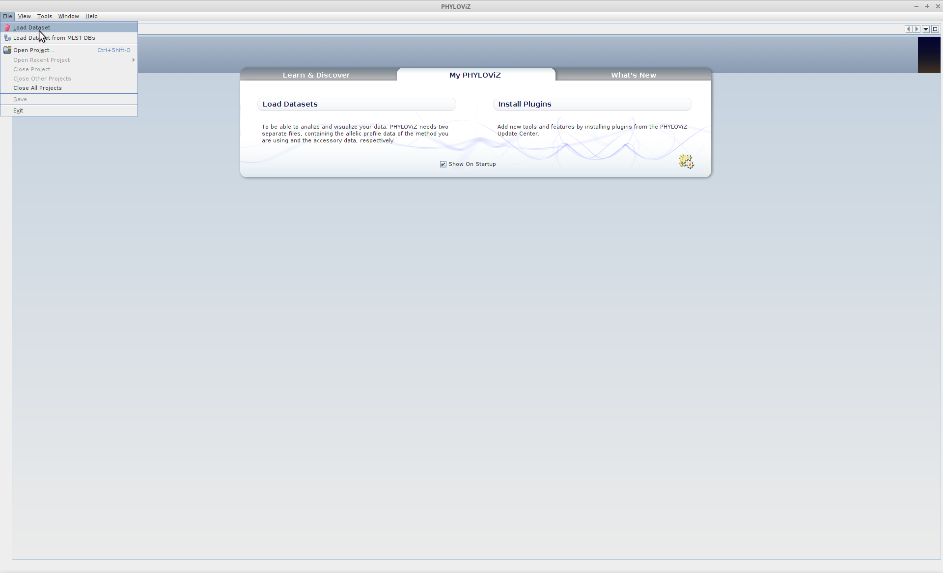
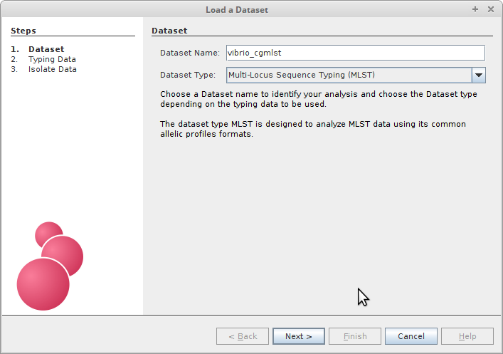
The first thing you’ll need to do of course is to load our newly defined cgMLST typing data into Phyloviz. Select the MLST analysis type from the dropdown menu, and we’ll give the analysis an informative name.

File --> Load Dataset

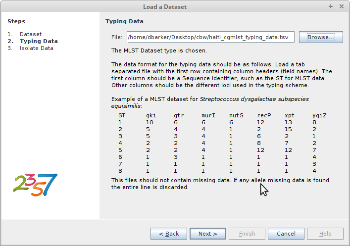
Next, load your typing data. In this case, our typing data is the table of core genome sequence types we created in R and saved to haiti_cgmlst_typing_data.tsv.

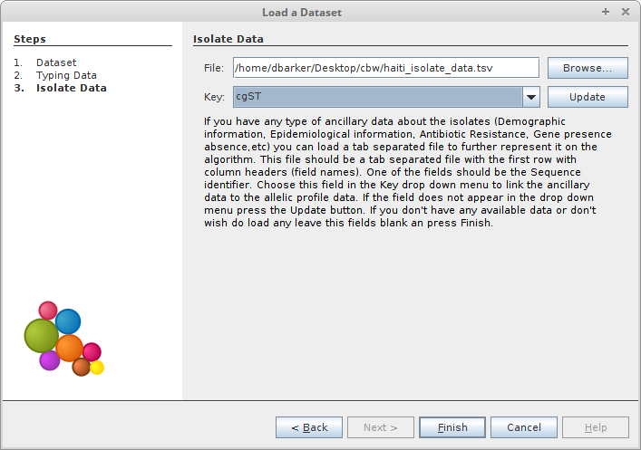
In order to get meaningful results from our cgMLST scheme, we’ll need to relate our cgSTs to the isolates they represent. To accomplish this, we’ll load the table of isolate data we created from our cgST definions and provenance data. We’ll be organizing the data on cgST, so select that as the key value.

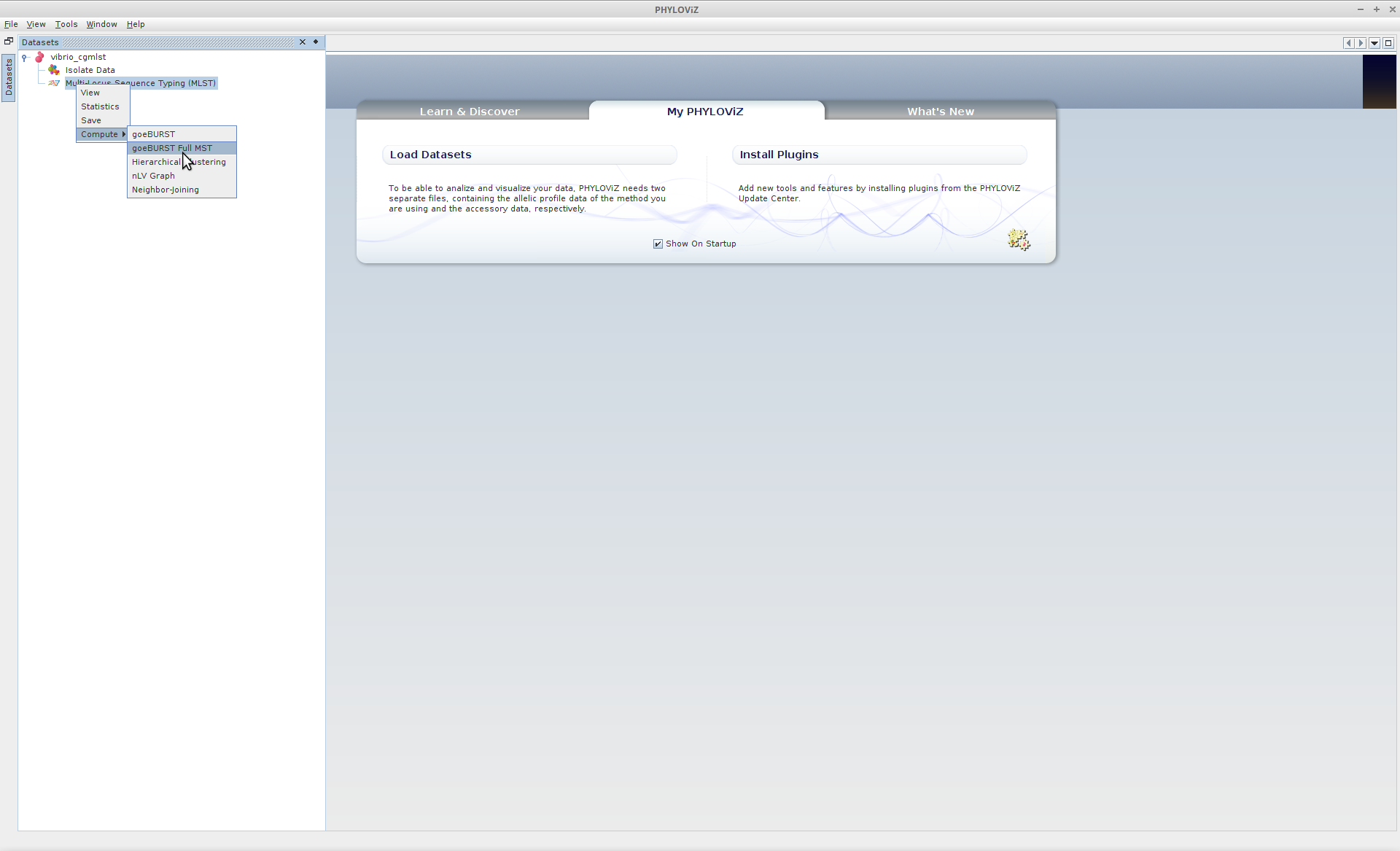
Now that all the data are loaded, we’ll calculate the globally optimal eBURST (goeBURST) clusters of the the dataset. Right-Click (Linux/Windows) or Ctrl-click (OS X) on the the typing data, and under “Compute” select goeBURST Full MST.

Multilocus Sequence Typing (MLST) --> Compute --> goeBURST Full MST

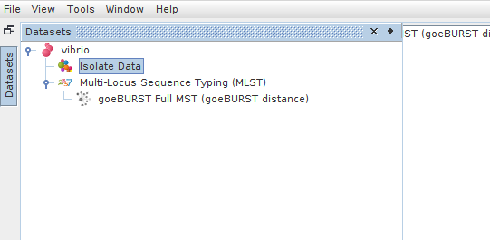
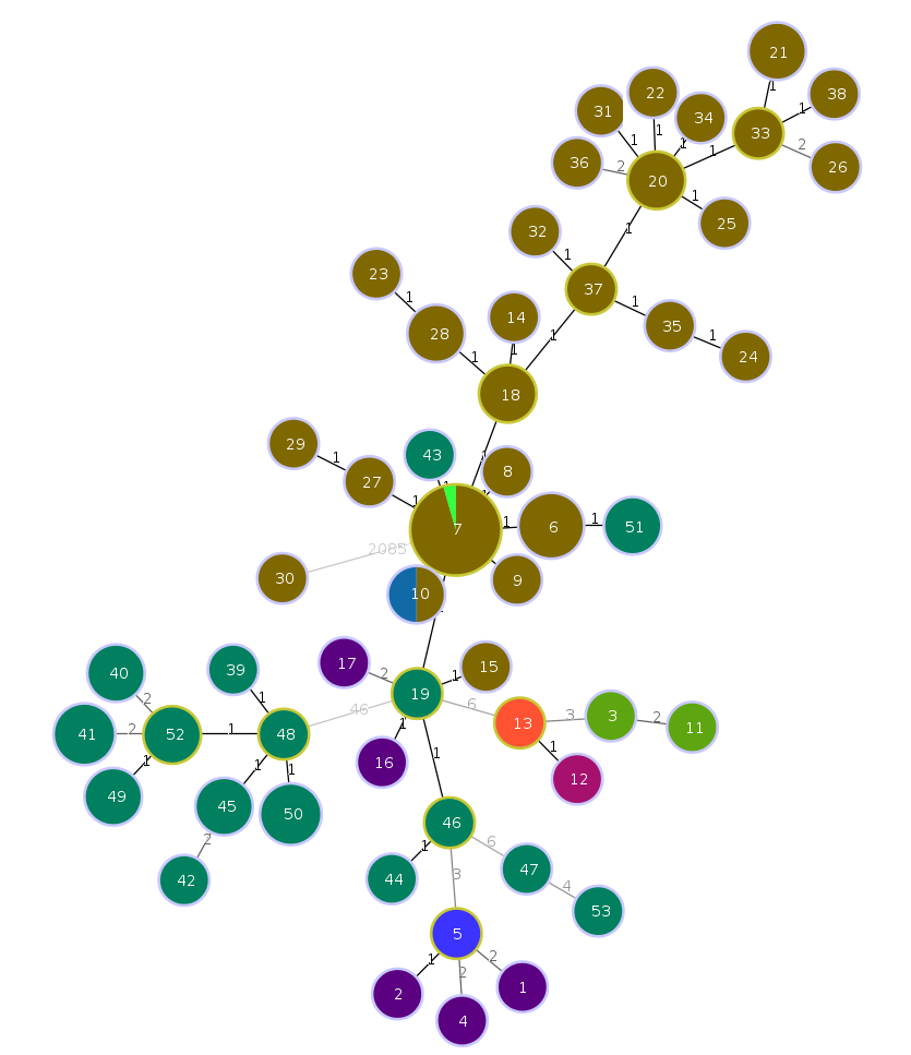
Once the MST calculation is complete (it should be very fast for a dataset of this size), expand “Multilocus Sequence Typing” and double-click where it says “goeBURST Full MST (goeBURST distance”

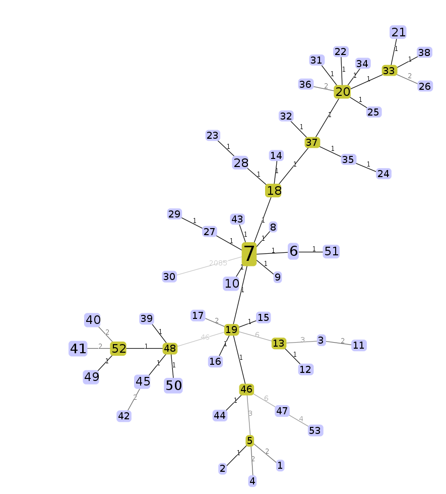
An interactive force-directed minimum spanning tree should be drawn and animating. Feel free to play around with it. Each node is labelled with the cgST name that it represents, and the size of each node is logarithmically scaled to the number of strains contained within the cgST. Edge lengths can be enabled under “Options” on the lower left of the screen.

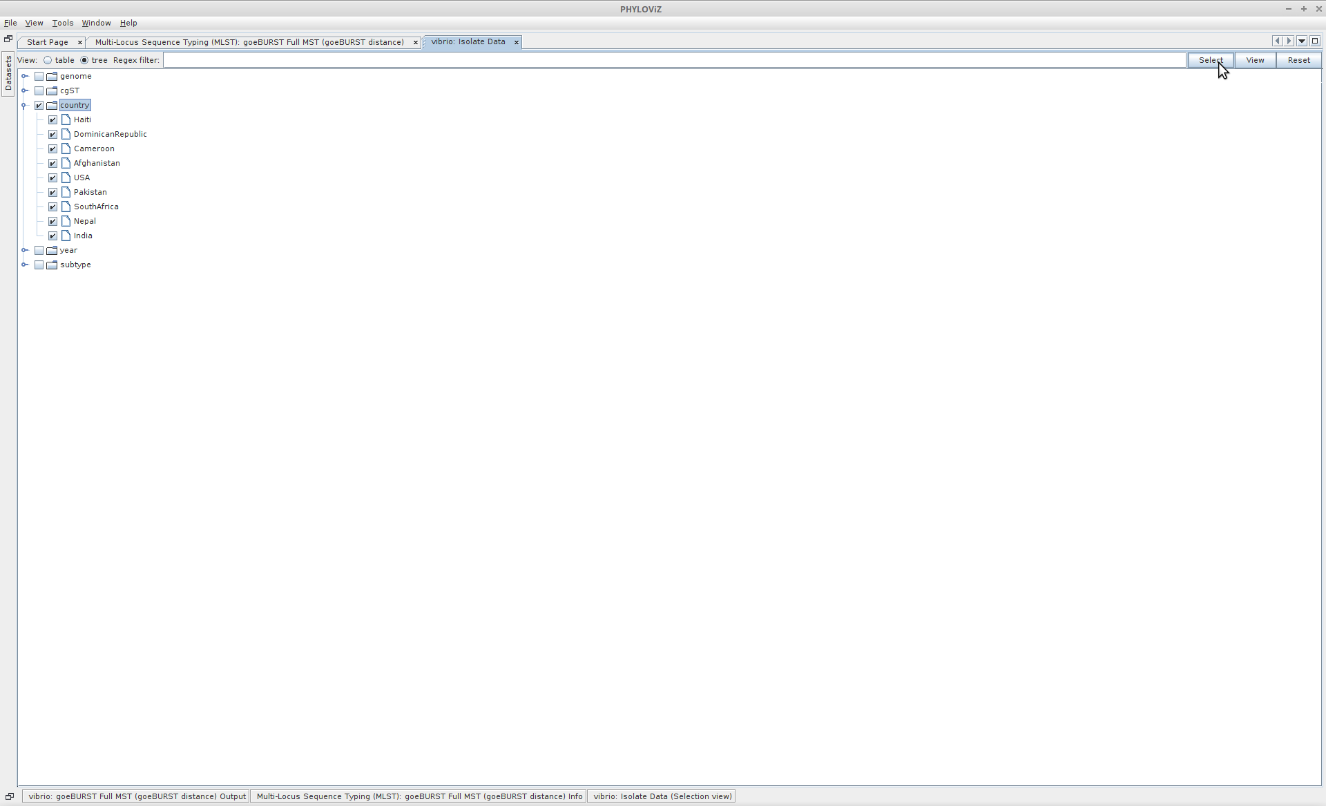
We can project any other data specified in the isolate data file as coloured annotations on the MST. Navigate to the isolate data tab. Select “Country” as a variable to project. Selecting the Tree option for viewing isolate data is often an easier method for selecting these variables. Once selected, click “View” in the upper right corner.

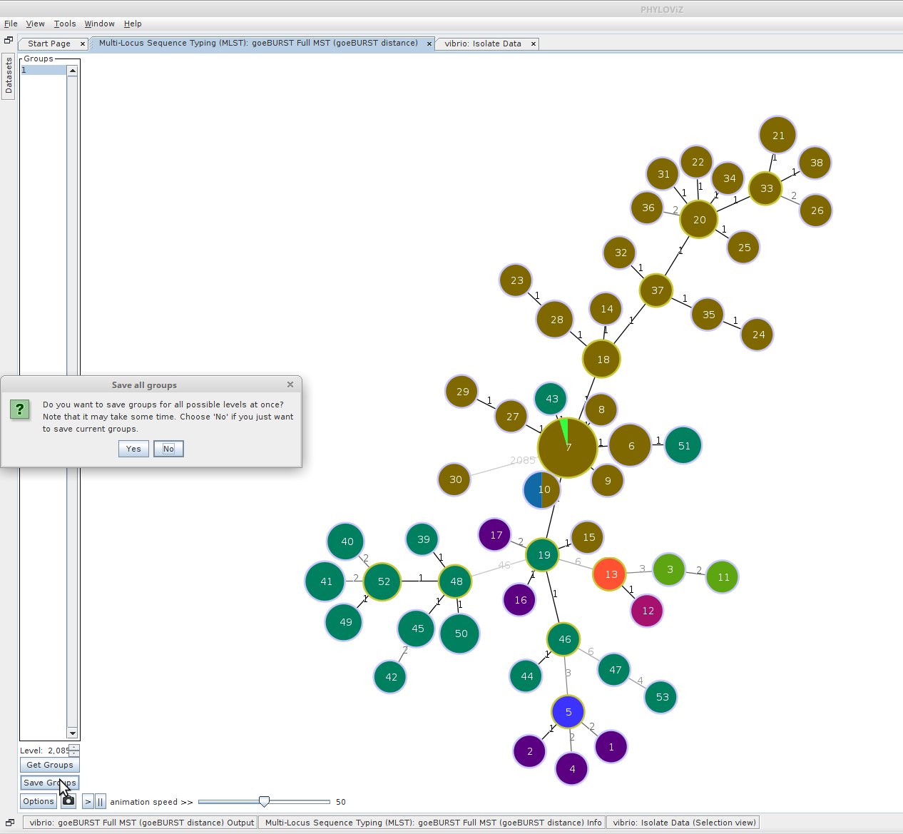
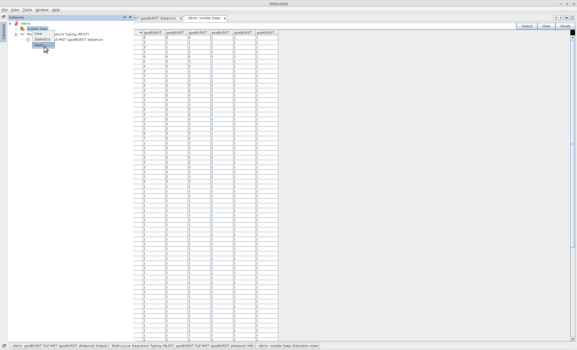
Finally we can use Phyloviz to cluster our strains into groups at each informative threshold. Toward the bottom-left of the screen, click “Save Groups”. When prompted, click “Yes” to save all groups at all goeBURST thresholds. These clusters will be saved back into your isolate data table. Your now-modified isolate data table can also be saved back into a file.

Adjusted Wallace Coefficient

The Adjusted Wallace Coefficient (AWC) is a metric that gives information about the relationship between two typing methods.

For typing methods A and B, if A -> B == 0.818 and B -> A == 0.559, this can be interpreted as,

“two strains clustered together by method A have a 81.8% probability of being clustered together by method B, while two strains grouped together by Method B have only a 59.9% probability of being clustered together by Method A.”

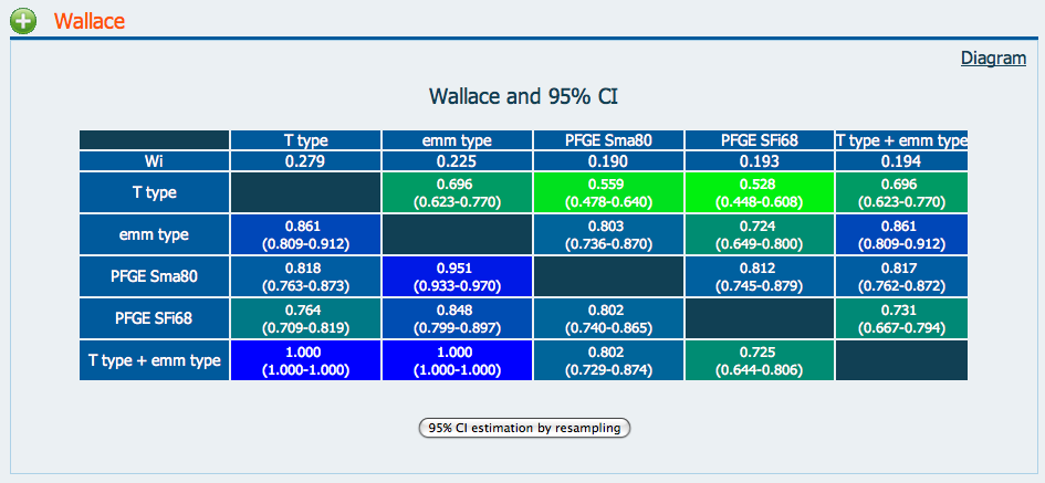
We can assess clustering methods relative to one another using the AWC. Comparing Partitions provides a convenient web tool for comparing microbial typing methods by AWC.

For example, we can compare the performance of classical 7-gene multilocus sequence typing with the various cgMLST thresholds. Conveniently, we can extact this information from or isolates

# we'll give slightly more informative column names to our isolate data first
sed -i 's/goeBURST MST\[\([0-9]*\)\]/cgmlst_\1/g' haiti_isolate_data.tsv

# Grab some potentially intesting colunms and filter out the unassigned
# MLST Sequence Types ("-")
cut -f 2,3,6,14-20 haiti_isolate_data.tsv | grep -v "-" > awc_typing_methods.tsv

Open awc_typing_methods.tsv in your favourite text editor and open http://www.comparingpartitions.info/index.php?link=Tool in a browser. Paste in your typing data and press Submit. You should see a matrix similar to the example above. Note that we included the “Country” column - the data provided need not necessarily be a typing method. cgST -> Country == 0.849!

Selecting a Robust Gene Subset

Now that we’ve selected a prototype cgMLST scheme, we should start to think about how robust this scheme will be in the future. It’s only been defined in terms of these particular genomes, after all. There are many problems associated with cgMSLT design using draft genome sequences, particularly incompletely sequenced genes (contig truncations), and the difficulty of determining whether a particular locus is biologically absent, or simply had insufficent coverage to be included in the assembly. These problems are often linearly associated with the length of sequence, i.e. the number of loci included in the scheme. A good solution for this is is to to use a robust subset of the core genome for your cgMLST scheme. But which subset?

For this last exercise, we’ll randomly select a small subset of 200 genes from our existing scheme (~10%). After selecting the genes, we’ll use Phyloviz to cluster our genomes using the new scheme, and finally we’ll find the AWC between our new scheme and the original using Comparing Partions. Sampling the genes will be random. Who will pick the “best” gene set that most closely recapitulates the full core genome?

See if you can put together the steps with what you’ve already learned. The tasks you’ll need to complete are:

• Randomly select 200 genes from our cgMLST scheme
• Define cgSTs for our cgMLST200
  • Export our new cgSTs to ~/workspace

Here’s the last snippet of R code you’ll need for the task.

# return randomly 200 column indices corresponding the your core genes
gene_selection_idx <- sample(seq_along(mtcars), 200)

core_subset <- core[, gene_selection_idx]

Done! Of course, this is a very brief look at cgMLST and the thought that goes into its design. It can be a very powerful tool, but it will require no small amount of effort work to design a robust, portable cgMLST scheme.