Pathway and Network Analysis of Omics Data Integrated Assignment
This work is licensed under a Creative Commons Attribution-ShareAlike 3.0 Unported License. This means that you are able to copy, share and modify the work, as long as the result is distributed under the same license.
Pathway and Network Analysis Integrated Assignment
By Veronique Voisin
Goal
Familiarize yourself with g:Profiler, GSEA , EnrichmentMap using the Esophageal adenocarcinoma gene expression data (DATASET 1). Familiarize yourself with ReactomeFI and GeneMANIA using mutation data (DATASET 2).
NOTE: Network layouts are flexible and can be rearranged. What you see when you perform these exercises may not be identical to what you see in the tutorial, or what you have seen other times that you have performed the exercises. Exact layouts and predictions can also be affected by updates to the networks database that GeneMANIA uses. However it is expected that the network weights and predicted genes will be similar to those shown here.
DATASET 1
Background
Gene expression data from Esophageal adenocarcinoma (EAC) is used for this first part of the integrated assignment. Esophageal adenocarcinoma (EAC) has a rising incidence and a 5-year survival of only 15%. The single major risk factor for development of EAC is chronic heartburn, which eventually leads to a change in the lining of the esophagus called Barrett’s Esophagus (BE).
Specimens were collected from patients with normal esophagus (NE) and Barrett’s esophagus (BE). RNA was extracted from these samples and expression profiling was assessed using Affymetrix HG-U133A microarray PMID:24714516. Differentially expressed genes between BE and NE were determined.

Data processing
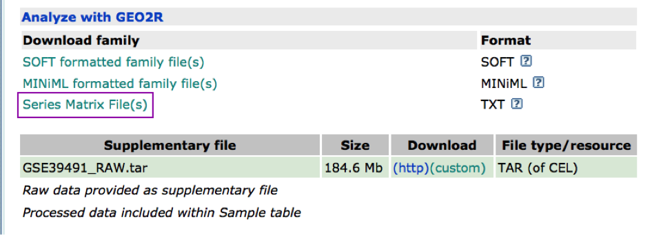
The Affymetrix data are stored in the Gene Expression Omnibus (GEO) repository under the accession number GSE39491 PMID:24714516. The RMA (Robust Multichip Average) normalized data were downloaded from GEO and further processed using the Bioconductor package limma to estimate differential expression between the groups. The results of the limma t-tests were corrected for multiple hypothesis testing using the Benjamini-HochBerg method (FDR).
For g:Profiler, genes with a FDR equal or less than 0.0001 and a logFC of 2 were retrieved and stored in a text file. For GSEA, a rank file has been created by ranking the genes from the highest t statistics value (up-regulated in BE compared to NE) to the lowest t values (down-regulated in BE compared to NE). The code used to process the data is available from the course page. Please feel free to adapt it and use it with your own data.
PART 1
-
Open g:Profiler
-
In Options, check Significantly only, No electronic GO annotations
-
Choose the databases: GO BP and Reactome.
-
Set minimum size of functional category to 3 and maximum to 500. Set 2 for the Size of query/ term intersection.
-
Set Benjamini-Hochberg as the significance threshold.
-
Run analysis of the genes differentially altered between BE and normal: copy and paste the gene list into the g:Profiler input window BEonly_genelist.txt.
-
Question: What is the most significant GO:term? What is the p-value for this GO:term?
-
Question: Is this p-value already corrected for multiple testing? What type of correction is used for your current analysis?
PART 2
- Re-run the analysis with User p-value threshold set to 0.0001. Question: What has been changed?
PART 3
An important feature of g:Profiler is an ability to work with sorted or ranked lists. The top of such a list is given more weight in determining the functional connections to GO:terms and/or pathways. Our gene list was initially sorted by the FDR value based on the significant differential expression.
-
Open g:Profiler in a new window and paste genes from BEonly_genelist.txt.
-
Use same options as part 2 (User p-value threshold set to 0.0001) and select also Ordered query.
-
Question: Do you seen any changes in the output in comparison to the analysis of the unordered gene list (PART 2)?
PART 4
Now we have to generate an output from the enrichment analysis and save it in appropriate format for EnrichmentMap. Please, change the output type to Generic Enrichment Map (TAB).
Run it using options used in PART 3. Download data in Generic EnrichmentMap (GEM) format. We will need this file for Enrichment map.
PART 5
Generate and save the Generic EnrichmentMap for genes in NConly_genelist.txt. It contains the genes specific of the normal tissue samples. Run g:Profiler with this list using same options as in PART 4 selecting Generic Enrichment Map (GEM) format as output type. We will need this file for EnrichmentMap.
PART 6
Create an EnrichmentMap to visualize the outputs from g:Profiler.
-
Open Cytoscape
-
Go: Apps > EnrichmentMap > Create Enrichment Map
- Let’s create an EnrichmentMap for the pathways that were enriched by the genes specific of the BE samples and one for the genes specific of the NC samples.
- Upload the files from your g:Profiler run (1 g:Profiler output file and the g:Profiler /gmt file, see module 2 lab if you need more instructions] into EnrichmentMap.
- Use the expression file BE_vs_NE_expression.txt file (right click, save link as). The expression file has to be uploaded in the “expression” field located above the “enrichment result” box.
- In parameters, use P-value Cutoff of 1 and FDR Q-value Cutoff of 0.05. Create 2 EnrichmentMaps, 1 for BE and 1 for NC
- Build the map.
-
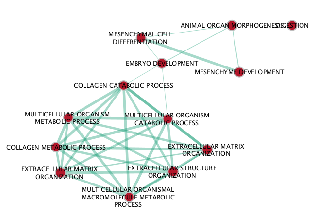
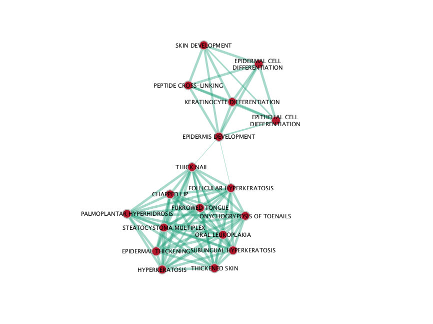
If successful, you will see a network where each node represents a pathway and edges connect pathways with shared genes. Node size is proportional to the number of genes in this pathway, intensity of the node color represents the enrichment strength and edge weight is relative to the number of genes shared between connected nodes.
-
Try different layouts. For example: Layouts -> yFiles Layouts -> Organic. Move nodes around to be able to read the labels.
-
Select a node of your choice. When the node is highlighted, the expression profile of all genes included in this pathway appears in the Heat Map (nodes) viewer tab. Get familiar with the options provided by this panel. Save expression Set.
-
Click on any edge (the line between nodes). In the Table panel ( Heat Map (edges)) you should see a heatmap of all genes both gene-sets connected by this edge have in common.
-
Select several nodes and edges. Heat Map (nodes) will show the union of all genes in the selected gene sets. Heat Map (edges) will show only those genes that all selected sets have in common.
- Go to View -> Show Results Panel. Change q-value (FDR) as well as similarity cutoffs and see how the network changes. Redo the layout. Save the file.
Question What conclusions can you make based on these networks?
BE map
NC map
Hint: you can obtain more gene-sets by using the gProfiler pvalue = 0.05 instead of 0.0001.
PART 7: GSEA
-
Launch GSEA.
-
Run GSEA using the rank file that has been created from the differential expression test comparing BE vs NE BEvsNE_ranks.rnk and the pathway file Human_GOBP_AllPathways_no_GO_iea_May_24_2016_symbol.gmt.
* open GSEA aas instructed in module 2
- upload the .rnk and .gmt files
- Use 100 permutations for the lab exercise /!\ but use 1000 for your own data analysis.
- Create an EnrichmentMap:
- look at module 3 if you don’t remember how to load the files. The enrichment results are 2 excel files called gsea_report_for_na_neg and gsea_report_for_na_pos within the GSEA folder saved on your computer. Tip: try the .rpt automatic upload : click on the enrichment field on the EnrichmentMap interface and locate the .rpt file in the GSEA folder.
- uses parameters a P-value Cutoff of 1 (in other words: we don’t use the pvalue filter), an FDR Q-value Cutoff of 0.001 and Jaccard Coefficient as Similarity Cutoff. Upload the expression file BE_vs_NE_expression.txt(right click, save link as).
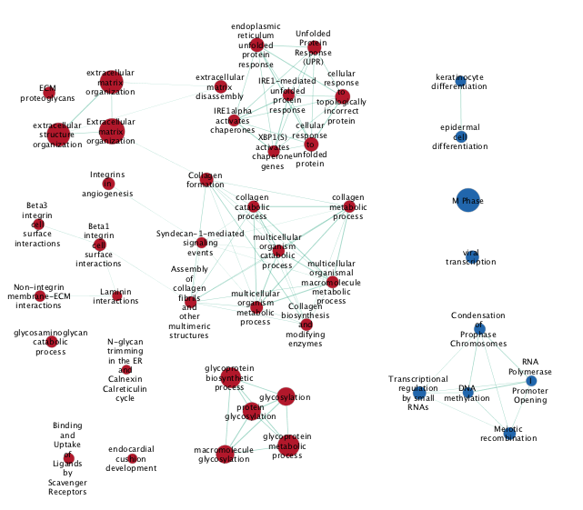
- Examine the results as you did for the g:Profiler map (e.g move nodes around, use the slide bar to adjust Q values). Save the file. Save an image.
DATASET 2
Stomach cancer or gastric cancer is a cancer developing from the lining of the stomach. The most common cause is infection by the bacteria Helicopter pylori, which accounts for more than 60% of cases. Certain types of ‘H. pylori’ have greater risks than others. Other common causes include eating pickled vegetables and smoking.
MutSig - is a mutation signal processing tool created by the Broad Institute. It estimates the significance of the gene mutation rate based on abundances of the mutations, clustering of the mutations in hotspots and conservation of the mutated positions.
The gene list for this assignment is the output from MutSig run based on Stomach Adenocarcinoma somatic mutations found in ~300 samples. It is publicly available through TCGA portal.
File provided: STAD_MutSig.txt
Goal: familiarize yourself with ReactomeFI and GeneMANIA.
PART 1
Create a network using ReactomeFI.
- Open Cytoscape.
- Choose App -> Reactome FI -> Gene set/mutation analysis
- Upload STAD_MutSig.txt and built a network without linkers:
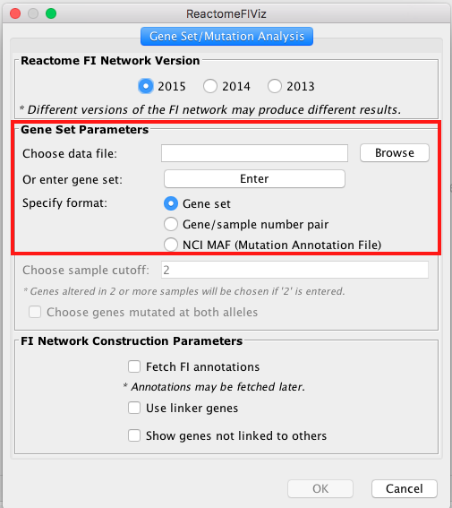 /!: the latest interface contains 2016 version of the ReactomeFI underlying database but this exercise has been prepared with the 2015 version. Please use the 2015 version to complete this exercise but the most up to date version when you work with your own data.

-
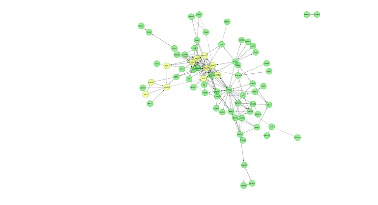
Fetch FI annotation (Hint: right click on a blank space, Reactome FI, Fetch FI Annotations). You should see arrows (directed graph).
-
Run Pathway enrichment (Hint: right click on the network panel and follow the path showed below). Question What is the pathway with the lowest (best) FDR?
-
Do a subnetwork of ErbB signaling pathway (K)
Hint:select the pathway in the table, that should highlight the genes in yellow. Use the subnetwork icon () on the tool bar to create it (“New network from selection”).
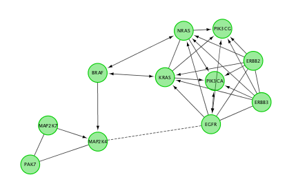
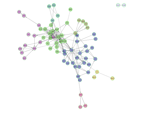
- Cluster the network and perform pathway enrichment on the network. Questions How many clusters did the analysis retrieve? What is the FDR value of the most significant pathway of module 0
PART 2
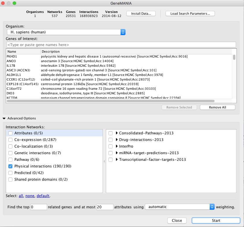
Use the same mutation data STAD_MutSig.txt to create a network using GeneMANIA in order to visualize which genes are known to physically interact with each other. Hint: select only “Physical interactions” in “Advanced Options” paramaters of the GeneMANIA input dialog box.
!Warning: Use the GeneMANIA Cytoscape app for this exercise. If you use it for the first time and you haven’t installed data as it was said in the installation instructions, only install “CORE” data as the full data may take 1 hour to download.
The network may look slightly different compared to above screenshots as the geneMANIA underlying pathway database has been recently updated.
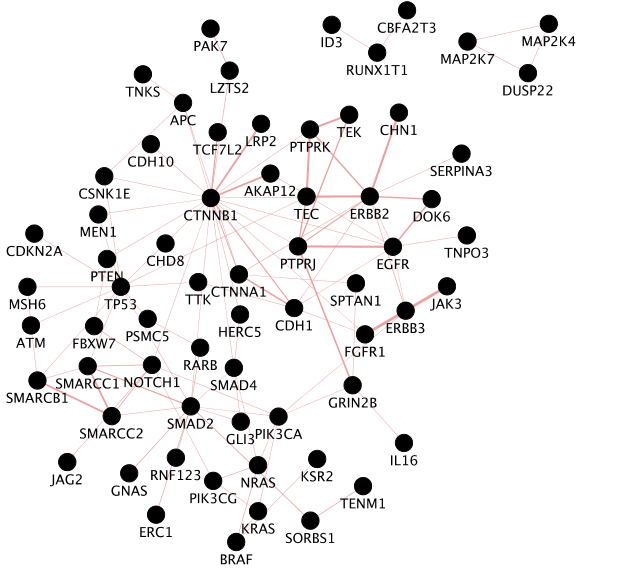
Locate CTNNB1, use the “First neighbors of selected nodes” icon in the tool bar to highlight genes connected to CTNNB1 and create a subnetwork. How many nodes do contain this subnetwork?
Hint: 
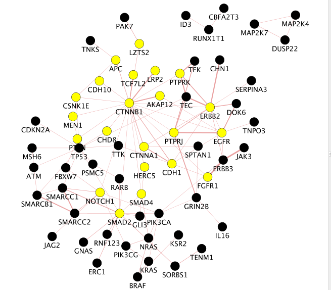
–
Congratulations! You have reached the end of the integrated assignment.