Cancer Analysis 2021
CAN Module 2 - Viewing cancer alignments in IGV
This lab is based on the HTS IGV lab originally by Sorana Morrissy and was updated and modified by Heather Gibling for the Cancer Analysis workshop.
Introduction
Description of the lab
Welcome to the lab for Genome Visualization! This lab will introduce you to the Integrative Genomics Viewer, a powerful desktop application for viewing many kinds of genomic data, including data for DNA sequencing, RNA sequencing, microarrays, epigenetics, and copy number alteration. It is one of the most popular visualization tools for high throughput sequencing (HTS) data.
After this lab, you will be able to:
- Very quickly navigate around the genome
- Visualize HTS read alignments
- Examine SNP calls and structural re-arrangements by eye
- Tell the difference between germline and somatic variants
Things to know before you start:
- The lab may take between 1-2 hours, depending on your familiarity with genome browsing. Don’t worry if you don’t complete the lab! It is available for you to complete later.
- There are a few thought-provoking Questions or Notes pertaining to sections of the lab. These are optional, and may take more time, but are meant to help you better understand the visualizations you are seeing.
Lab components
- Visualization Part 1: Getting familiar with IGV
- Visualization Part 2: Inspecting small variants in the normal sample
- Visualization Part 3: Inspecting small somatic variants in the tumor sample
- Visualization Part 4: Inspecting structural variants in NA12878
Requirements
- Integrative Genomics Viewer
- Ability to run Java
Compatibility
This tutorial was last tested on IGV v2.9, which is available on the Download page. It should work for versions as old as v2.3, but it is strongly recommended that you use a newer version to take advantage of new features and better performance.
Data Set for IGV
These bams are a sneak peak of the ones you will be creating in module 3. They are a renal cancer tumor-normal matched pair from the CageKid project.
Download the files to your computer in one directory (folder) and unzip them. Remember where you saved them!
Visualization Part 1: Getting familiar with IGV
The IGV Interface

Load a Genome and Data Tracks
By default, IGV loads Human hg19 as the reference genome. If you work with another version of the human genome, or another organism altogether, you can change the genome by clicking the drop down menu in the upper-left.
We will also load additional tracks from Server (File -> Load from Server):
- GC Percentage
- dbSNP 1.4.7


Navigation
You should see a listing of chromosomes in this reference genome. Click on 1, for chromosome 1.

Navigate to chr1:10,000-11,000 by entering this into the location field (in the top-left corner of the interface) and clicking Go or pressing Enter/Return on your keyboard. This shows a window of chromosome 1 that is 1,000 base pairs wide and beginning at position 10,000.
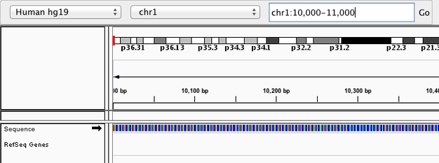
IGV displays the sequence of letters in a genome as a sequence of colours (e.g. A = green). This makes repetitive sequences, like the ones found at the start of this region, easy to identify.
You can navigate to a gene of interest by typing it in the same box the genomic coordinates are in and pressing Enter/Return. Try it for your favourite gene, or BRCA1 if you can’t decide.
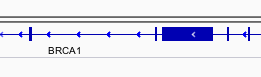
Genes are represented as lines and boxes. Lines represent intronic regions, and boxes represent exonic regions. The arrows indicate the strand on which the gene lies.
When loaded, tracks are stacked on top of each other. You can identify which track is which by consulting the label to the left of each track.
Region Lists
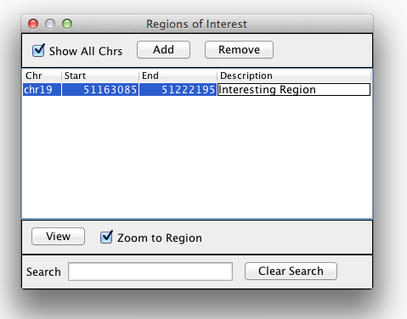
Sometimes it’s really useful to save where you are, or to load regions of interest. For this purpose, there is a Region Navigator in IGV. To access it, click Regions > Region Navigator. While you browse around the genome, you can save some bookmarks by pressing the Add button at any time. Add a useful label in the Description box to help you remember why you saved the region later on.
Loading Read Alignments
We will first visualize alignments from the subset of normal sample. In IGV choose File > Load from File, select normal.bam, and click OK. Note that the bam and index (bam.bai) files must be in the same directory for IGV to load these properly, but only the bam file needs to be loaded into IGV.

Visualizing Read Alignments
Navigate to a narrow window on chromosome 9: “chr9:130,620,912-130,621,487”.
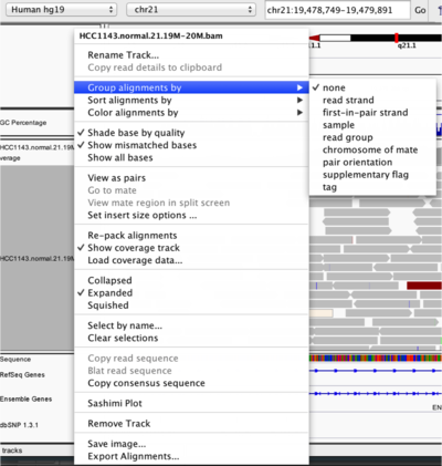
IGV lets you group, sort, and color alignments to better visualize the data. To start our exploration, right click on the track name (normal.bam), and select the following options:
- Sort alignments by start location
- Group alignments by pair orientation
Experiment with the various settings by right clicking the read alignment track and toggling the options. Think about which would be best for specific tasks (e.g. quality control, SNP calling, CNV finding).
You can also change how many reads are visible in the track by changing their width. Rick click the normal.bam track name and test out Collapsed, Expanded, and Squished. Collapsed or Expanded is recommended for this lab.
A handy tool is the center line. In the menu bar, go to View > Preferences > Alignments and check the box for Show center line (you might have to scroll down a bit). This is useful when you want to sort alignments by a specific base (e.g. at a SNP site) for making sure you are sorting on the correct base.

You will see reads represented by grey or white bars stacked on top of each other, where they were aligned to the reference genome. The reads are pointed to indicate their orientation (i.e. the strand on which they are mapped). By default, individual bases are only colored if they are a mismatch to the reference. The transparacy of the mismatched bases corresponds to the base quality (essentially how confident we are that the sequencing machine called the correct base).

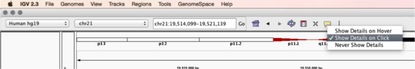
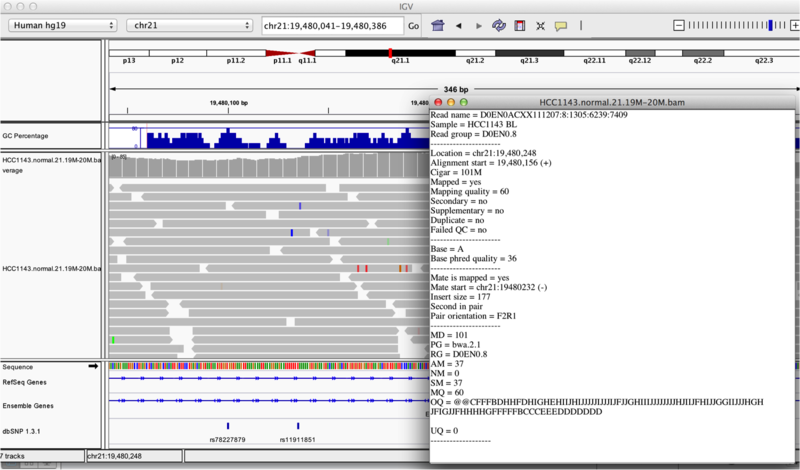
Mouse over or click on any read and notice that a lot of information is available. To toggle read display from hover to click, select the yellow box at the top of the window and change the setting.
Once you select a read, a pop-up window shows quality metrics and other information about that read (if your setting is on click but you don’t see a popup box, they might be hiding behind the IGV window or on the other screen if you have a two-screen setup). We will learn more about these metrics in Module 3.
Visualization Part 2: Inspecting small variants in the normal sample
Heterozygous and Homozygous SNPs
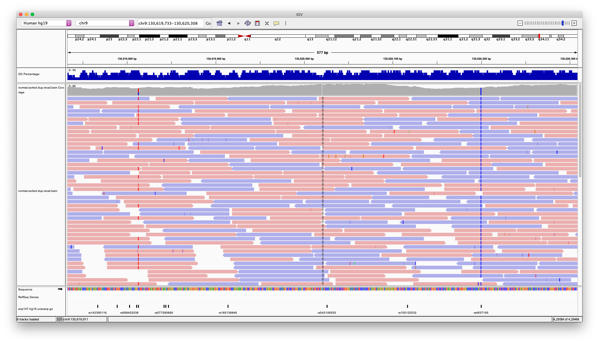
- Navigate to chr9:130619733-130620308
- Which variant is heterozygous and which is homozygous?
- What are the variant allele frequencies for each SNP? To find out you can click/hover on the colored bars in the coverage track
- Now color alignments by read strand. Red reads are in the forward orientation, and blue reads are in the reverse orientation.
- Do these look like true SNPs? What evidence is there for this?
- Look at the other mismatched bases in the region between the two SNPs.
- Are these sequencing errors, SNPs, or SNVs?
- What does Shade base by quality do and how might this be helpful?
- Can a normal sample have somatic SNVs?
Homozygous deletion
- Navigate to chr9:130555407-130556072

- How large is this deletion?
- Is it homozygous or heterozygous?
GC coverage
- Navigate to chr9:130284240-130286902

- What do you notice about the coverage track and GC Percentage track?
- What does coloring alignments by read strand tell you?
- Do you think this is a deletion? Compare this region to the previous region.
Visualization Part 3: Inspecting small somatic variants in the tumor sample
Load tumor.bam the same way you loaded normal.bam. You can resize the tracks to make them both fit better as needed by dragging the horizontal line between the samples up and down.
Somatic SNV
- Navigate to chr9:130633300-130633965

- How many SNVs are in this region for each sample?
- What is the variant allele frequency for the extra SNV in the tumor sample? How did it get this high?
Somatic SNP with change in heterozygosity
- Navigate to chr9:130515234-130515399 and sort alignments by base

- What are the variant allele frequencies for each sample?
- Why are these frequencies different?
Somatic indel next to SNP with change in heterozygosity
- Navigate to chr9:130337723-130337888 and sort alignments by base

- What type of variant is in the centre?
- In the normal sample there is a SNP to the right. What do you notice about this variant in the tumor sample?
- What might be an explanation for what happened?
Visualization Part 4: Inspecting structural variants in NA12878
Cancers often have large structural variants, like inversions, duplications, and translocations. We will examine some structural variants in a well-studied individual (NA12878) from the Platinum Genomes Project. Note that this is a normal sample, but think about how these variants might look in a tumor sample.
First remove the coverage and alignment tracks for both the tumor and normal samples. Click on the top coverage track, then hold down the shift key and click on the bottom alignment track. The four tracks should now be grey. Right click anywhere on the tracks and select Remove Tracks.

Now go to File > Load from server and click on the arrow next to Platinum Genomes to expand the selection. Click on NA12878 (second from the top).

The IGV User Guide has great explanations of how we can use colorings by pair orientation or insert size to view structural variants.
Inversion
- Navigate to chrX:14728136-14732366 and make the following viewing adjustments:
- Select View as pairs
- Group alignments by pair orientation
- Color alignments by pair orientation
- Sort alignments by start location

- What do you notice about the blue and teal reads at the top?
- How does View as pairs help understand that this is an inversion?
- Is this inversion heterozygous or homozygous?
Duplication
- Navigate to chr17:55080031-55081661, sort alignments by start location, and keep the same viewing options as the previous inversion

- What do you notice about the green reads at the top?
- Note: Green reads when colored by read orientation can indicate a translocation as well as a duplication. If you zoom out you can see there is a rise in the coverage track above the green reads, suggesting this is a duplication of the sequence at this location.
Large deletion
- Navigate to chr7:39811931-39833535 and color alignments by insert size, keeping the other options the same. Sort by start location

- What do the red read pairs indicate?
- What other track can we look at to see that this is a deletion?
You’re done! We hope that you enjoyed the lab and that you continue to enjoy IGV.
If you want to look at more examples, check out this IGV lab from CBW’s Highthroughput Sequencing Data workshop!