Cancer Analysis 2021 Module 4
================================
This work is licensed under a Creative Commons Attribution-ShareAlike 3.0 Unported License. This means that you are able to copy, share and modify the work, as long as the result is distributed under the same license.
================================
In this workshop, we will work with common tools to process and analyze cancer sequencing data. Using the command line we will analyze DNA sequencing from the whole genome. The focus of this workshop will be on calling single nucelotide variants, insertion, deletions (commonly referred to as SNV/indels) as well as calling copy-number variations (CNVs). We will also annotate SNV & CNV files, such that we will known the functional consequence of these variants.
Data Source: we will be working on the CageKid samples from Module3. Whole genome sequencing and analysis can take multiple days to run, as such we have downsampled the files so that we can proceed in a timely fashion.
The tools and their general function we are going to using for calling SNV’s and CNV’s are:
- mutect2 –> SNV/INDEL variant calling
- varscan2 –> SNV/INDEL variant calling
- samtools –> Bam manipulation
- bcftools –> vcf manipulation
- bgzip and tabix –> compress and index
- annovar –> annotation
- controlfreec –> CNV calling
- bedtools –> segment manipulation
- awk –> line by line file manipulation
- R & R-Studio –> visualization
Files for variant calling:
1) Bam –> Sequence alignments from Module3 or /home/ubuntu/CourseData/CAN_data/Module4/alignments/normal/normal.sorted.realigned.bam
2) Reference genome –> /home/ubuntu/CourseData/CAN_data/Module4/references/human_g1k_v37.fasta
3) Germline-reference file –> /home/ubuntu/CourseData/CAN_data/Module4/accessory_files/Homo_sapiens.GRCh37.gnomad.exomes.r2.0.1.sites.no-VEP.nohist.tidy.vcf.gz
This germline reference file is from the Gnomad database of germline variation in the human population. It includes the variant allele frequency and known single nucleotide polymorphisms thereby providing a starting probability that the sample carries the allele in the germline.
Part 1, step 1 Running Mutect2
cd ~/workspace
mkdir -p Module4_somaticvariants
cd  ~/workspace/Module4_somaticvariants
/usr/local/GATK/gatk Mutect2 -R /home/ubuntu/CourseData/CAN_data/Module4/references/human_g1k_v37.fasta -I /home/ubuntu/CourseData/CAN_data/Module4/alignments/normal/normal.sorted.dup.recal.bam -I /home/ubuntu/CourseData/CAN_data/Module4/alignments/tumor/tumor.sorted.dup.recal.bam -normal normal -tumor tumor -O pairedVariants_mutect2.vcf -L 9:130215000-130636000 --germline-resource /home/ubuntu/CourseData/CAN_data/Module4/accessory_files/Homo_sapiens.GRCh37.gnomad.exomes.r2.0.1.sites.no-VEP.nohist.tidy.vcf.gz
Question: The -normal and -tumor are represented by which field in the bam?
samtools view /home/ubuntu/CourseData/CAN_data/Module4/alignments/tumor/tumor.sorted.dup.recal.bam | head -n 1 | less -S
side note: Mutect2 can also take multiple samples. In this case you only have to specify the normal sample! how neat is that!
This will generate an initial variant call format file. This is a standardized way in which variants are reported. For a full description of the vcf_format:
Every VCF has three sections Metadata, Header and variants. The Metadata
less pairedVariants_mutect2.vcf | egrep '##' | less -S
##fileformat=VCFv4.2
##FORMAT=<ID=AD,Number=R,Type=Integer,Description="Allelic depths for the ref and alt alleles in the order listed">
##FORMAT=<ID=AF,Number=A,Type=Float,Description="Allele fractions of alternate alleles in the tumor">
##FORMAT=<ID=DP,Number=1,Type=Integer,Description="Approximate read depth (reads with MQ=255 or with bad mates are filtered)">
##FORMAT=<ID=F1R2,Number=R,Type=Integer,Description="Count of reads in F1R2 pair orientation supporting each allele">
##FORMAT=<ID=F2R1,Number=R,Type=Integer,Description="Count of reads in F2R1 pair orientation supporting each allele">
##FORMAT=<ID=GQ,Number=1,Type=Integer,Description="Genotype Quality">
##FORMAT=<ID=GT,Number=1,Type=String,Description="Genotype">
##FORMAT=<ID=PGT,Number=1,Type=String,Description="Physical phasing haplotype information, describing how the alternate alleles are phased in relation to one another">
##FORMAT=<ID=PID,Number=1,Type=String,Description="Physical phasing ID information, where each unique ID within a given sample (but not across samples) connects records within a phasing group"> The Header ``` less pairedVariants_mutect2.vcf | egrep '#CHROM' | less -S ```
#CHROM  POS     ID      REF     ALT     QUAL    FILTER  INFO    FORMAT  normal  tumor The Variants ``` less pairedVariants_mutect2.vcf | egrep -v '#' | head -n1 ```
9       130219144       .       CA      C       .       .       DP=89;ECNT=1;MBQ=32,32;MFRL=284,277;MMQ=60,60;MPOS=25;NALOD=1.09;NLOD=5.79;POPAF=6.00;RPA=15,14;RU=A;STR;TLOD=4.79   GT:AD:AF:DP:F1R2:F2R1:SB        0/0:22,1:0.042:23:6,1:12,0:14,8,1,0     0/1:25,4:0.157:29:9,4:9,0:17,8,3,1
Question: What is the definition of AD and AF in this mutect2-VCF?
The pairedVariants_mutect2.vcf does not contain any filter information. Filter information comes from each variant and generates tags we can use to filter these mutations.
gatk FilterMutectCalls -R /home/ubuntu/CourseData/CAN_data/Module4/references/human_g1k_v37.fasta --filtering-stats pairedVariants_mutect2.vcf.stats -V pairedVariants_mutect2.vcf -O pairedVariants_mutect2_filtered.vcf
Let’s look at our file now.
less -S pairedVariants_mutect2_filtered.vcf | egrep -v '#' | less -S
We can see in the FILTER column there are now filters
less -S pairedVariants_mutect2_filtered.vcf | egrep -v '#' | cut -f 1,2,4,5,7 | less -S
Question: what does the “germline” in the FILTER field mean?
Since we will be comparing with another tool it is best to try to consider as many sites as possible. To this end we will be using bcftools:
bcftools --help
bcftools norm --help
bcftools norm will help us here
1) Split multiallelic (Ref == A & Alt == AT,ATT) into two seperate variants A –> AT and A –> ATT
2) It will ensure we are left-aligned. Which is a way to normalize variants based on the reference genome. (https://github.com/bioinformatics-ca/CAN_2021/blob/main/Module4/Data/Normalization_mnp.png)
bcftools norm -m-both -f /home/ubuntu/CourseData/CAN_data/Module4/references/human_g1k_v37.fasta -Oz -o pairedVariants_mutect2_filtered_normalized.vcf.gz pairedVariants_mutect2_filtered.vcf
tabix pairedVariants_mutect2_filtered_normalized.vcf.gz
Question: what does -m-both accomplish here
Part 1, step 2:
Running varscan2 (http://varscan.sourceforge.net/)
First we create pileup files from both the normal sample and the control sample. This is done with a tool called samtools:
samtools mpileup -B -q 1 -f /home/ubuntu/CourseData/CAN_data/Module4/references/human_g1k_v37.fasta -r 9:130215000-130636000 /home/ubuntu/CourseData/CAN_data/Module4/alignments/tumor/tumor.sorted.realigned.bam > tumor.mpileup
samtools mpileup -B -q 1 -f /home/ubuntu/CourseData/CAN_data/Module4/references/human_g1k_v37.fasta -r 9:130215000-130636000 /home/ubuntu/CourseData/CAN_data/Module4/alignments/normal/normal.sorted.realigned.bam > normal.mpileup
A pileup contains the information of every single base-pair. Simply put this consolidates our data to help varscan call variants. The first three columns are the pretty obvious (chromosome, postion and reference) The fourth column is the number of reads covering the site The fifth and sixth are the read-bases and the base qualities
less -S tumor.mpileup
Next we use varscan2 to execute the somatic function which does the initial variant calling from our mpileups. For parameters here we are setting a strand-filter to 1 meaning we will remove variants that are favored by >90% on one strand. We are also setting a p-value threshold of the variant being somatic to 0.05.
java -Xmx2G -jar /usr/local/VarScan.v2.3.9.jar somatic normal.mpileup tumor.mpileup --output-vcf 1 --strand-filter 1 --somatic-p-value 0.05 --output-snp varscan2.snp.vcf --output-indel varscan2.indel.vcf
Question: What is the definition of AD and RD in this varscan-VCF & how would you calculate the variant allele frequency?
less -S varscan2.snp.vcf
We now set the minimum variant allele frequency to 0.05 or 5%. Two default parameters are also indicated by examining the function with –help
java -Xmx2G -jar /usr/local/VarScan.v2.3.9.jar processSomatic --help
java -Xmx2G -jar /usr/local/VarScan.v2.3.9.jar processSomatic varscan2.indel.vcf --min-tumor-freq 0.05
java -Xmx2G -jar /usr/local/VarScan.v2.3.9.jar processSomatic varscan2.snp.vcf --min-tumor-freq 0.05
This will split our varscan.snp.vcf and varscan.indel.vcf into 6 files each.
LOH.vcf & LOH.hc.vcf Germline.vcf & Germline.hc.vcf Somatic.vcf & Somatic.hc.vcf The hc.vcf indicate that there is a higher confidence that these variants are somatic. We want to work with the best set of variant calls so we selected the *hc.vcf.
LOH: stands for Loss of heterozygozity. Meaning we had a region with A and B allele and lost the mix of A and B.
Question: What happened in the LOH variant below?
#CHROM  POS     ID      REF     ALT     QUAL    FILTER  INFO    FORMAT  NORMAL  TUMOR
9       130311404       .       A       C       .       PASS    DP=125;SS=3;SSC=28;GPV=1E0;SPV=1.4873E-3        GT:GQ:DP:RD:AD:FREQ:DP4                     0/1:.:71:32:39:54.93%:20,12,23,16        1/1:.:54:10:44:81.48%:6,4,27,17
Question: What happened in the LOH variant below?
9 130346618 . G A . PASS DP=49;SS=3;SSC=32;GPV=1E0;SPV=5.4288E-4 GT:GQ:DP:RD:AD:FREQ:DP4 0/1:.:26:10:16:61.54%:5,5,5,11 0/0:.:23:20:3:13.04%:5,15,1,2
Question: In what cancer type would having germline variants be useful?
Zip and tabix of high confidence variants. Bcftools concat wants to work with zipped files
bgzip varscan2.snp.Somatic.hc.vcf
tabix varscan2.snp.Somatic.hc.vcf.gz

bgzip varscan2.indel.Somatic.hc.vcf
tabix varscan2.indel.Somatic.hc.vcf.gz
Combine high-confidence snp and indels.
bcftools concat allows us to combine vcf’s from the same sample, it is not the same as bcftools merge. -a allows us to have overlaps such as a snp and indel occurring in the same location.
bcftools concat -Oz -a -r 9:130215000-130636000 varscan2.snp.Somatic.hc.vcf.gz varscan2.indel.Somatic.hc.vcf.gz -o pairedVariants_varscan2_filtered.vcf.gz
Again let’s normalize
bcftools norm -m-both -f /home/ubuntu/CourseData/CAN_data/Module4/references/human_g1k_v37.fasta -Oz -o pairedVariants_varscan2_filtered_normalized.vcf.gz pairedVariants_varscan2_filtered.vcf.gz
tabix pairedVariants_varscan2_filtered_normalized.vcf.gz
Part 1, step 3
Now we have finished variant calling using two different variants callers. The next step is to combine the output of the multiple callers.
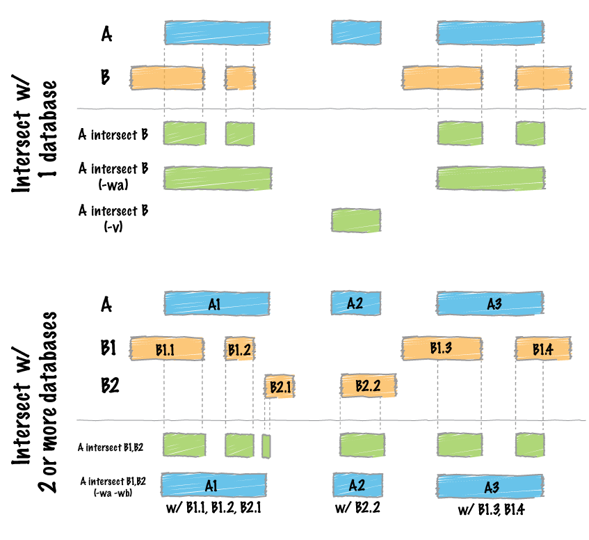
bcftools isec --help
bcftools isec -n+1 -f PASS -p intersectionDirectory pairedVariants_mutect2_filtered_normalized.vcf.gz pairedVariants_varscan2_filtered_normalized.vcf.gz
This creates a directory named intersectionDirectory that contains all variants that pass in at-least one vcf. It’s at this point where you can choose which variants to include.
cd ~/workspace/Module4_somaticvariants/intersectionDirectory/
- All variants – The union includes all variants and has a low false negative count but a high false positives count
- Common variants – The intersection is the subset of high confidence varianta with fewer false positive and potentially more false negatives.
In this directory we see the 0000.vcf and 0001.vcf. These corresponds to the mutect2 vcf and the varscan2 vcf, respectively. (confirmed in the README.txt)
If we review the sites.txt files:
less -S sites.txt
9       130223126       C       T       01
9       130264057       T       A       11
9       130296899       A       T       11
9       130308743       C       A       11
This reads that the first variants on chromosme 9, position 130223126 changes from a C to a T:, This variant was called in the varscan.vcf (01). 11 corresponds to the being called in both and 10 is being called in only mutect2.
less -S sites.txt | cut -f 5 | sort | uniq -c
  4 01
  6 10
 11 11
This show’s us that varscan2 has 4 unique variants, mutect2 has 6 unique variants and there are 11 shared variants.
Let’s combine our mutect2 and varscan2 vcfs into a single vcf. This will generate the union of variants.
cd ~/workspace/Module4_somaticvariants
bcftools merge -f PASS pairedVariants_mutect2_filtered_normalized.vcf.gz pairedVariants_varscan2_filtered_normalized.vcf.gz -o pairedVariants_mutect2_varscan2.vcf.gz -Oz
Now that we have our two vcf’s combined we can look at their contents.
Every vcf has a metadata sections two ##
zless -S pairedVariants_mutect2_varscan2.vcf.gz | egrep '##' | head -n 10
  ##fileformat=VCFv4.2
  ##FILTER=<ID=PASS,Description="All filters passed">
  ##FILTER=<ID=FAIL,Description="Fail the site if all alleles fail but for different reasons.">
  ##FILTER=<ID=base_qual,Description="alt median base quality">
  ##FILTER=<ID=clustered_events,Description="Clustered events observed in the tumor">
  ##FILTER=<ID=contamination,Description="contamination">
  ##FILTER=<ID=duplicate,Description="evidence for alt allele is overrepresented by apparent duplicates">
  ##FILTER=<ID=fragment,Description="abs(ref - alt) median fragment length">
  ##FILTER=<ID=germline,Description="Evidence indicates this site is germline, not somatic">
  ##FILTER=<ID=haplotype,Description="Variant near filtered variant on same haplotype.">
This section contains details about the vcf including:
- Explanations of the FILTERS, INFO and FORMAT.
- Contigs used and their length
- Processes taken to generate the vcf eg bcftools_mergeCommand=merge -o pairedVariants_mutect2_varscan2.vcf.gz -Oz 0000.vcf.gz 0001.vcf.gz
Every vcf has a column (with one #) and
less -S pairedVariants_mutect2_varscan2.vcf.gz | egrep '#CHROM' | head -n 1
CHROM POS ID REF ALT QUAL FILTER INFO FORMAT normal tumor NORMAL TUMOR
The header has 8 mandatory columns. CHROM, POS, ID, REF, ALT, QUAL, FILTER & INFO
These are followed by a FORMAT column header and sample ID’s. These sample id’s will follow from their vcf’s. In our case mutect2 (normal tumor) and then varscan2 (NORMAL TUMOR)
Every vcf has a content section which has the variants.
less -S pairedVariants_mutect2_varscan2.vcf.gz | egrep -v '#' | head -n 1
9 130223126 . C T . PASS SOMATIC;SS=2;SSC=18;GPV=1;SPV=0.014587;DP=55 GT:GQ:DP:RD:AD:FREQ:DP4 ./.:.:.:.:.:.:. ./.:.:.:.:.:.:. 0/0:.:26:26:0:0%:14,12,0,0 0/1:.:29:22:6:21.43%:15,7,1,5
This shows a variant on chromosome 9 position 130223126 that goes from the reference C to a T. This variant was called uniquely by varscan2. This variant has passed all filters. The INFO and FORMAT field has additional information that can be explained in more detail using the ‘##’ information. Please note that missing data is denoted as a ‘.’.
Annotating our combined files
mkdir -p ~/workspace/Module4_somaticvariants/results
annovar is a tool to annotate our vcf files with gene names & functional information. There are a number of different [annovar_databases]https://annovar.openbioinformatics.org/en/latest/user-guide/download/)
/usr/local/annovar/table_annovar.pl pairedVariants_mutect2_varscan2.vcf.gz /usr/local/annovar/humandb/ -buildver hg19 -out results/annotated_mutect2_varscan2 -remove -protocol refGene -operation g -nastring . --vcfinput
This will produce two annotation files: annotated_mutect2_varscan2.hg19_multianno.vcf & annotated_mutect2_varscan2.hg19_multianno.txt. These files contain the gene annotations and infer the functional consequence of each variant.
The header for contains the vcf fields but they have been renamed by annovar. However now we can see which genes are affected and how they are changed.
cd /home/ubuntu/workspace/Module4_somaticvariants/results
less annotated_mutect2_varscan2.hg19_multianno.txt | head -n 1 | sed 's/\t/|/g'
Chr|Start|End|Ref|Alt|Func.refGene|Gene.refGene|GeneDetail.refGene|ExonicFunc.refGene|AAChange.refGene|Otherinfo1|Otherinfo2|Otherinfo3|Otherinfo4|Otherinfo5|Otherinfo6|Otherinfo7|Otherinfo8|Otherinfo9|Otherinfo10|Otherinfo11|Otherinfo12|Otherinfo13|Otherinfo14|Otherinfo15|Otherinfo16
For example our first variant is an intronic mutation in LRSAM1.
9 130223126 130223126 C T intronic LRSAM1 . . . 0.25 . 31 9130223126 . C T . PASS SOMATIC;SS=2;SSC=21;GPV=1;SPV=0.0064791;DP=55 GT:GQ:DP:RD:AD:FREQ:DP4 ./.:.:.:.:.:.:. ./.:.:.:.:.:.:. 0/0:.:24:24:0:0%:13,11,0,0 0/1:.:31:23:8:25.81%:17,6,3,5
less -S annotated_mutect2_varscan2.hg19_multianno.txt | cut -f 6 | sort | uniq -c
This shows the genomic region change where each variant is occuring. Typically exonic variants are more likely to produce a phenotypic change.
     1 Func.refGene
     5 exonic
     1 intergenic
    15 intronic
less -S annotated_mutect2_varscan2.hg19_multianno.txt | cut -f 9 | sort | uniq -c
     16 .
      1 ExonicFunc.refGene
      2 frameshift insertion
      3 nonsynonymous SNV
This shows the functional consequence of each exonic variant, we have 5 exonic variants that results in two frameshifts and 3 nonsynonymous SNV’s.
Next we can examine some variants in IGV.
start IGV ensure hg19 is selected
load your bam files by clicking file –> load from file If you have not downloaded the bam or are missing it. It is provided here (https://drive.google.com/drive/folders/1f_1pDbpNaNUT6oC-pEPXInemyZwMV4Hc)
Input: chr9:130634110


Here we can see evidence of the C –> T in the tumor bam but not in the normal sample. This variant is called correctly and is called by both mutect2 and varscan2.
9 130634110 130634110 C T exonic AK1 nonsynonymous_SNV 0/0:48,0:0.02:48:22,0:26,0:21,27,0,0:.:.:.:. 0/1:50,30:0.376:80:25,10:25,19:26,24,14,16:.:.:.:. 0/0:0:.:47:.:.:.:.:47:0%:21,26,0,0 0/1:29:.:79:.:.:.:.:50:36.71%:26,24,15,14
Now input chr9:130634993.
 Here we can see evidence of two variants in the AKT1 exonic region. These variants are called only using mutect2.
If you can’t see the variants. In IGV go to View –> Preferences –> Alignments then change Coverage allele-fraction threshold to 0.1 (10%)
9       130634993       130634993       C       T       exonic  AK1     nonsynonymous SNV       0/0:46,0:0.021:46:24,0:21,0:18,28,0,0   0/1:48,8:0.155:56:24,5:24,3:20,28,5,3   ./.:.:.:.:.:.:. ./.:.:.:.:.:.:.
9       130635011       130635011       C       G       exonic  AK1     nonsynonymous SNV       0/0:39,0:0.024:39:23,0:16,0:17,22,0,0   0/1:46,9:0.175:55:21,5:25,4:16,30,5,4   ./.:.:.:.:.:.:. ./.:.:.:.:.:.:.
Question: Compare the variant allele frequency between these three variants in AK1. Which one’s came first?
Now input chr9:130316821. This will be an intronic variant in the NIBAN2 gene.

9 130316821 130316821 C T intronic NIBAN2 . ./.:.:.:.:.:.:. ./.:.:.:.:.:.:. 0/0:.:23:20:0:0%:13,7,0,0 0/1:.:24:19:5:20.83%:14,5,1,4
Question: This variant is only called by varscan2, what red flags exist for this variant?
Short break time
part 2, step 1
Copy number variations
In this workshop, we will present the main steps for calling copy number variations (CNVs). Normally we would perform a copy number variation analysis on alignment files (BAMs). Due to time and resource constraints we will not be able to do this analysis on the full sequence or from shortened bam files. Instead we will be working with some preprocessed data using gc correction files and mpileups. Our data sample is again the cagekid sample c0098.
To examine the copy number states within the cage kid tumors we are going to be using a tool called [controlfreec] (http://boevalab.inf.ethz.ch/FREEC/)
With this tool we can call
- Copy number gains
- Copy number losses
- Copy-neutral loss of heterozygosity
- This tool can also be used on exome seqencing and can even be used without a control (non-tumor) sample.
controlfreec requires the sequence data and these additional files
- A reference genome and a reference index (fasta and fai):
- List of single nucelotide polymorphisms
Running controlfreec
cd ~/workspace/Module4_somaticvariants
mkdir -p copynumber
cd ~/workspace/Module4_somaticvariants/copynumber
The first step is to generate a configuration file which contains the parameters and file locations.
bash /home/ubuntu/CourseData/CAN_data/Module4/scripts/generate_controlfreec_configurationfile.sh > CBW_config.txt
Let’s now look at the configuration file.
less CBW_config.txt
###Controlfreec has many different parameters
In the config file has four categories: general, sample, control and BAF.
I have commented out the BAM files, however if you you were running this for the first time you should start from the BAM file. Instead we use pileups and gc content.
- pileup contain base-pair information which we discussed earlier.
-
gc content for normalization between normal and tumor.
- [General] indicates parameters for how we want the algorithm to run; parameters like minCNAlength, intercept are indicating WGS is being used
- [sample] indicates the input data of our tumor either in bam format or pileup/cpn
- [control] indicates our input data of our normal sample, again in different formats
- [BAF] indicates the necesarry files for calculatibng the b-allele frequency which will help us identify regions of LOH
#Now to run controlfreec
/usr/local/bin/freec -conf CBW_config.txt > output.log
please note here we will get some warning that segmentation is not-completed, this due to subsetting the files to allow for a quicker runtime.
Let’s list the files we generated here.
ls *
 CBW_regions_c0098_Tumor.sorted.markduplicates.bam_sample.cpn_BAF.txt : Containing the allele frequency
 CBW_regions_c0098_Tumor.sorted.markduplicates.bam_sample.cpn_ratio.txt : Contain read-depth ratios
 CBW_regions_c0098_Tumor.sorted.markduplicates.bam_sample.cpn_CNVs : Containing our copy numbers calls
 CBW_regions_c0098_Tumor.sorted.markduplicates.bam_sample.cpn_info.txt : Containing sample information, purity and ploidy   ```  less CBW_regions_c0098_Tumor.sorted.markduplicates.bam_sample.cpn_info.txt  ```
Question: The purity is suggested to be 100% do you think we have enough information to say this?
While we don’t have annovar we can intersect our segment file with a gene transfer format file or [GTF] (http://m.ensembl.org/info/website/upload/gff.html). We will introduce awk and bedtools here. 1) awk is a command line tool that allows for command line manipulations of files (https://www.shortcutfoo.com/app/dojos/awk/cheatsheet) 2) bedtools allows for us to manipulate based on genomic regions (chr start end) which is the format of .BED files!
bedtools intersect which is a way to subset regions to the common regions between to bed files. It is useful for seeing what belongs to a particular region.
bedtools intersect -wb -b <(less CBW_regions_c0098_Tumor.sorted.markduplicates.bam_sample.cpn_CNVs | awk 'NF==7' | awk '{print "chr"$1"\t"$2"\t"$3"\t"$0}' | less -S) -a <(less /home/ubuntu/CourseData/CAN_data/Module4/accessory_files/Homo_sapiens.GRCh37.Ensemble100.FullGeneAnnotations.txt | awk '$4=="ensembl_havana"') | awk '{print $1"\t"$2"\t"$3"\t"$7"\t"$8"\t"$15}' > AnnotatedCBW_regions_c0098_Tumor.sorted.markduplicates.bam_CNVs.tsv
less -S AnnotatedCBW_regions_c0098_Tumor.sorted.markduplicates.bam_CNVs.tsv
We can examine a gene of interest, such as a loss of VHL which is common in kidney cancers.
less AnnotatedCBW_regions_c0098_Tumor.sorted.markduplicates.bam_CNVs.tsv | awk '$4=="VHL"' | less -S
Now lets go visualize these results using R –> You will need to open r studio for this, we have two ways to do this. 1) Open it locally on you personal computer 2) In your url enter “http://your IPv4 or your IPv4 DNS:8080” —> then enter your username: ubuntu and your password
This script is available with controlfreec but due to the subsettting we will have to plot the ratio and BAF ourselves.
- If you are missing any of the data it can be found at github
- https://github.com/bioinformatics-ca/CAN_2021/raw/main/Module4/Data/CBW_regions_c0098_Tumor.sorted.markduplicates.bam_sample.cpn_BAF.txt
- https://github.com/bioinformatics-ca/CAN_2021/raw/main/Module4/Data/CBW_regions_c0098_Tumor.sorted.markduplicates.bam_sample.cpn_ratio.txt
Let’s read in our data
ratio_dataTable <- read.table(file = "/home/ubuntu/workspace/Module4_somaticvariants/copynumber/CBW_regions_c0098_Tumor.sorted.markduplicates.bam_sample.cpn_ratio.txt", header=TRUE)
#ratio_dataTable <- read.table(file = "https://github.com/bioinformatics-ca/CAN_2021/raw/main/Module4/Data/CBW_regions_c0098_Tumor.sorted.markduplicates.bam_sample.cpn_ratio.txt",header=TRUE)

ratio <- data.frame(ratio_dataTable)
BAF_dataTable <-read.table(file="/home/ubuntu/workspace/Module4_somaticvariants/copynumber/CBW_regions_c0098_Tumor.sorted.markduplicates.bam_sample.cpn_BAF.txt", header=TRUE)
#BAF_dataTable <- read.table(file = "https://github.com/bioinformatics-ca/CAN_2021/raw/main/Module4/Data/CBW_regions_c0098_Tumor.sorted.markduplicates.bam_sample.cpn_BAF.txt"", header=TRUE)
BAF<-data.frame(BAF_dataTable)
ploidy <- 2
Now we can plot all of our data in a way that allows us to see gain, losses and neutral regions
for (chrom in c(3))
{
tt <- which(ratio$Chromosome==chrom)
if (length(tt)>0)
{
        plot(ratio$Start[tt],log2(ratio$Ratio[tt]),xlab = paste ("position, chr",chrom),ylab = "normalized copy number profile (log2)",pch = ".",col = colors()[88],cex=4)
        tt <- which(ratio$Chromosome==chrom  & ratio$CopyNumber>ploidy )
        points(ratio$Start[tt],log2(ratio$Ratio[tt]),pch = ".",col = colors()[136],cex=4)

        tt <- which(ratio$Chromosome==chrom  & ratio$CopyNumber<ploidy & ratio$CopyNumber!= -1)
        points(ratio$Start[tt],log2(ratio$Ratio[tt]),pch = ".",col = colors()[461],cex=4)
        tt <- which(ratio$Chromosome==chrom)
        }
        tt <- which(ratio$Chromosome==chrom)
}
This code below will plot our BAF plots
for (i in c(3))
{
tt <- which(BAF$Chromosome==i)
if (length(tt)>0)
  {
                lBAF <-BAF[tt,]
                plot(lBAF$Position,lBAF$BAF,ylim = c(-0.1,1.1),xlab = paste ("position, chr",i),ylab = "BAF",pch = ".",col = colors()[1])

                tt <- which(lBAF$A==0.5)
                points(lBAF$Position[tt],lBAF$BAF[tt],pch = ".",col = colors()[92])
                tt <- which(lBAF$A!=0.5 & lBAF$A>=0)
                points(lBAF$Position[tt],lBAF$BAF[tt],pch = ".",col = colors()[62])
                tt <- 1
                pres <- 1

                if (length(lBAF$A)>4) {
                        for (j in c(2:(length(lBAF$A)-pres-1))) {
                                if (lBAF$A[j]==lBAF$A[j+pres]) {
                                        tt[length(tt)+1] <- j
                                }
                        }
                        points(lBAF$Position[tt],lBAF$A[tt],pch = ".",col = colors()[24],cex=3)
                        points(lBAF$Position[tt],lBAF$B[tt],pch = ".",col = colors()[24],cex=3)
                }

                tt <- 1
                pres <- 1
                if (length(lBAF$FittedA)>4) {
                        for (j in c(2:(length(lBAF$FittedA)-pres-1))) {
                                if (lBAF$FittedA[j]==lBAF$FittedA[j+pres]) {
                                        tt[length(tt)+1] <- j
                                }
                        }
  points(lBAF$Position[tt],lBAF$FittedA[tt],pch = ".",col = colors()[463],cex=3)
  points(lBAF$Position[tt],lBAF$FittedB[tt],pch = ".",col = colors()[463],cex=3)
}}}
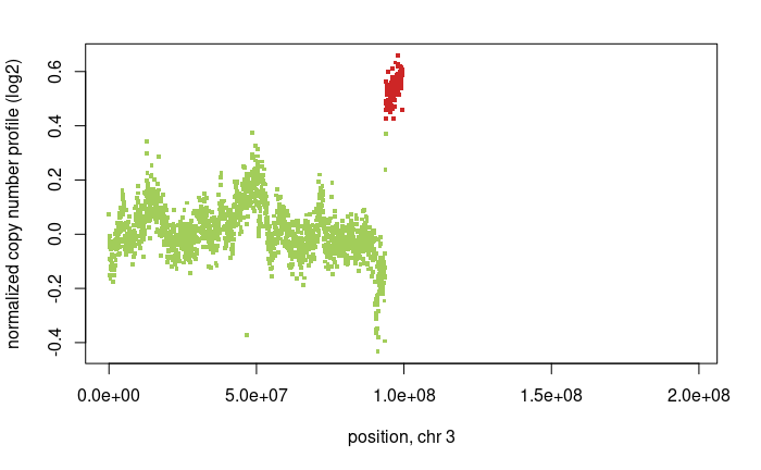
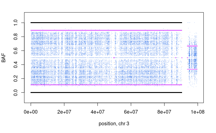
Question: What does each dot mean in the top CNV plots and what does each dot mean in the bottom BAF plot?
Question: What is the absolute copy-number of the red region in the top plot?
Question: Comparing the green region to the BAF plots, what kind of copy number variation is taking place?
Using a completed CNV calling on WGS data from the Terry Fox Research Initiative on GBM we can see how it looks across a whole genome. TFRI-WGS
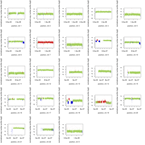
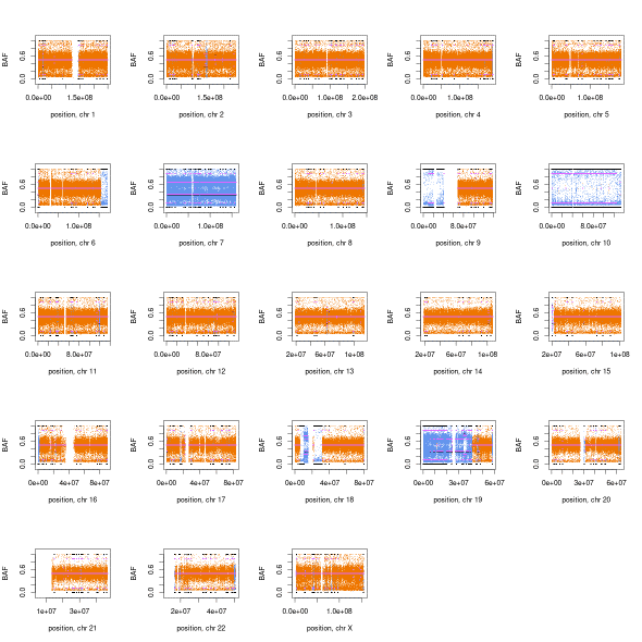
Question: What CNV events are supported by the data?
Question: There are hundred of segments as seen in both CNV and BAF plots, what is one way you can modify controlfreec to call fewer segments?
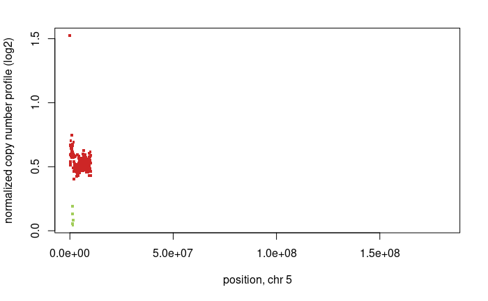
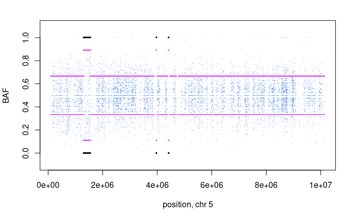
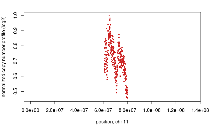
We can also plot chromosome 5 regions and chromosome 11 regions
for (chrom in c(5,11))
{
tt <- which(ratio$Chromosome==chrom)
if (length(tt)>0)
{
        plot(ratio$Start[tt],log2(ratio$Ratio[tt]),xlab = paste ("position, chr",chrom),ylab = "normalized copy number profile (log2)",pch = ".",col = colors()[88],cex=4)
        tt <- which(ratio$Chromosome==chrom  & ratio$CopyNumber>ploidy )
        points(ratio$Start[tt],log2(ratio$Ratio[tt]),pch = ".",col = colors()[136],cex=4)

        tt <- which(ratio$Chromosome==chrom  & ratio$CopyNumber<ploidy & ratio$CopyNumber!= -1)
        points(ratio$Start[tt],log2(ratio$Ratio[tt]),pch = ".",col = colors()[461],cex=4)
        tt <- which(ratio$Chromosome==chrom)
        }
        tt <- which(ratio$Chromosome==chrom)
}
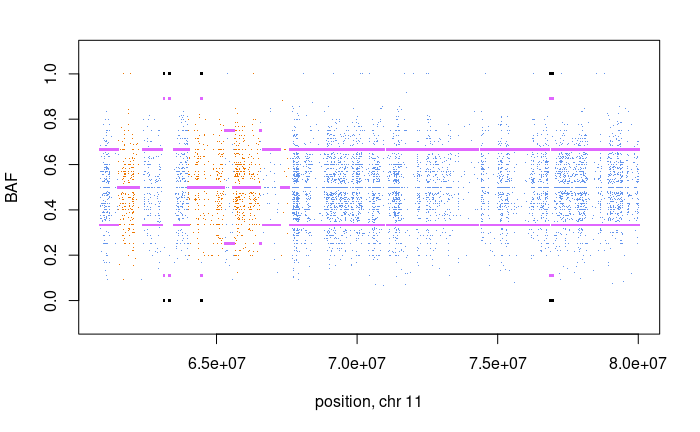
for (i in c(5,11))
{
tt <- which(BAF$Chromosome==i)
if (length(tt)>0)
  {
                lBAF <-BAF[tt,]
                plot(lBAF$Position,lBAF$BAF,ylim = c(-0.1,1.1),xlab = paste ("position, chr",i),ylab = "BAF",pch = ".",col = colors()[1])

                tt <- which(lBAF$A==0.5)
                points(lBAF$Position[tt],lBAF$BAF[tt],pch = ".",col = colors()[92])
                tt <- which(lBAF$A!=0.5 & lBAF$A>=0)
                points(lBAF$Position[tt],lBAF$BAF[tt],pch = ".",col = colors()[62])
                tt <- 1
                pres <- 1

                if (length(lBAF$A)>4) {
                        for (j in c(2:(length(lBAF$A)-pres-1))) {
                                if (lBAF$A[j]==lBAF$A[j+pres]) {
                                        tt[length(tt)+1] <- j
                                }
                        }
                        points(lBAF$Position[tt],lBAF$A[tt],pch = ".",col = colors()[24],cex=3)
                        points(lBAF$Position[tt],lBAF$B[tt],pch = ".",col = colors()[24],cex=3)
                }

                tt <- 1
                pres <- 1
                if (length(lBAF$FittedA)>4) {
                        for (j in c(2:(length(lBAF$FittedA)-pres-1))) {
                                if (lBAF$FittedA[j]==lBAF$FittedA[j+pres]) {
                                        tt[length(tt)+1] <- j
                                }
                        }
  points(lBAF$Position[tt],lBAF$FittedA[tt],pch = ".",col = colors()[463],cex=3)
  points(lBAF$Position[tt],lBAF$FittedB[tt],pch = ".",col = colors()[463],cex=3)
}}}
Now we see a chromsome 5 region which represents a gain and it is supported by the BAF
And we also see another gain on chromsome 11, which is again supported by the BAF.
### Special thanks to Dr.Morrissy & Dr.Bourgey for access to the CAGEKID data and access to genpipes ###
Answers (https://github.com/bioinformatics-ca/CAN_2021/blob/main/Module4/Answer_readme.txt)