Module 4: Single Nucleotide Variant Calling
Lab
Introduction
The goal of this practical session is to identify single nucleotide variants (SNVs) in a human genome and to annotate them. In the previous module 3, we have aligned the reads from NA12878 (daughter) in a small region on chromosome 1. We will continue to use the data generated during the Module 3.
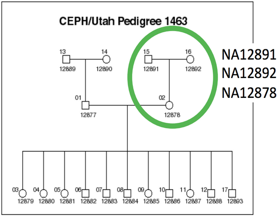
NA12878 is the child of the trio while NA12891 and NA12892 are her parents.
For practical reasons we subsampled the reads from the sample because running the whole dataset would take way too much time and resources. We’re going to focus on the reads extracted from a 300 kbp stretch of chromosome 1
| Chromosome | Start | End |
|---|---|---|
| 1 | 17704860 | 18004860 |
Original Setup
Software Requirements
These are all already installed, but here are the original links.
In this session, we will particularly focus on GATK HaplotypeCaller SNV detection tool. The main advantage of HaplotypeCaller is to do the calling using a local de-novo assembly approach. When the program encounters a region showing signs of variation, it discards the existing mapping information and completely reassembles the reads in that region. This allow a better accuracy in regions that are traditionally difficult to call, for example when they contain different types of variants close to each other.
Environment setup
mkdir -p $HOME/workspace/HTG/Module4/

docker run --privileged -v /tmp:/tmp --network host -it -w $PWD -v $HOME:$HOME \
--user $UID:$GROUPS -v /etc/group:/etc/group  -v /etc/passwd:/etc/passwd \
-v /etc/fonts/:/etc/fonts/ -v /media:/media c3genomics/genpipes:0.8

export WORK_DIR_M4=$HOME/workspace/HTG/Module4/
export REF=$MUGQIC_INSTALL_HOME/genomes/species/Homo_sapiens.GRCh37/
mkdir -p ${WORK_DIR_M4}/bam/NA12878
cd $WORK_DIR_M4

ln -s ~/CourseData/HTG_data/Module4/* .
cp $HOME/workspace/HTG/Module3/alignment/NA12878/NA12878.sorted.ba* bam/NA12878
cp $HOME/workspace/HTG/Module3/alignment/NA12878/NA12878.sorted.dup.recal.ba* bam/NA12878


module load mugqic/java/openjdk-jdk1.8.0_72 mugqic/GenomeAnalysisTK/4.1.0.0 mugqic/snpEff/4.3
Data files
The initial structure of your folders should look like this:
ROOT
|-- bam/               # bam file from the previous Module(down sampled)
    `-- NA12878/             # Child sample directory
`-- scripts/                 # command lines scripts
`-- saved_results/ # precomputed final filesInput files
Let’s look into the NA12878 bam folders.
ls bam/NA12878/Our starting data set consists of 100 bp paired-end Illumina reads from the child (NA12878) that have been aligned to GRCh37 during one of the previous modules (NA12878.sorted.bam). We also have the same data after duplicate removal, indel realignment and base recalibration (NA12878.sorted.dup.recal.bam).
1. Do you know what are the .bai files?
Solution (click here)
A bai file is an indexed form of a bam - it’s a companion to your bam that contains the index.
A bam file is a binary blob that stores all of your aligned sequence data. The index allows to acces specific region of the bam file without having to decompress the data and read it from start.
Working with indexed bam file allows to speed-up the data acces. Moreover many tools require index bam files.
Calling Variants with GATK
If you recall from the previous module, we first mapped the reads to GRCh37 and then we removed duplicate reads and realigned the reads around the indels.
Let’s call SNPs in NA12878 using both the original and the improved bam files:
mkdir -p variants
#NA12878.sort
java -Xmx2g -jar $GATK_JAR HaplotypeCaller \
-R $REF/genome/Homo_sapiens.GRCh37.fa \
-I bam/NA12878/NA12878.sorted.bam \
-O variants/NA12878.hc.vcf \
-L 1:17704860-18004860

#NA12878.sort.rmdup.realign
java -Xmx2g -jar $GATK_JAR HaplotypeCaller \
-R $REF/genome/Homo_sapiens.GRCh37.fa \
-I bam/NA12878/NA12878.sorted.dup.recal.bam \
-O variants/NA12878.rmdup.realign.hc.vcf \
-L 1:17704860-18004860
-Xmx2g instructs java to allow up 2 GB of RAM to be used for GATK.
-R specifies which reference sequence to use.
-I specifies the input BAM files.
-L indicates the reference region where SNP calling should take place
Investigating the SNP Calls
Use less to take a look at the vcf files:
less -S variants/NA12878.rmdup.realign.hc.vcfVcf is a daunting format at first glance, but you can find some basic information about the format [here](https://www.internationalgenome.org/wiki/Analysis/vcf4.0.
Fields vary from caller to caller. Some values are more constant. The ref vs alt alleles, variant quality (QUAL column) and the per-sample genotype (GT) values are almost always there.
1. How do you figure out what the genotype is for each variant?
Solution (click here)
Genotypes are given per individuals in the 10+ columns.
Based on the FORMAT description, the genotype (GT) is the first information provided (separated by :).
3 different values are available:
- 0/0 : homozgote reference (with the REF columns value)
- 1/1 : homozgote variant (with the ALT columns value)
- 1/0 : heterozygote (with both REF and ALT columns values)
2. Do we have any annotation information yet?
Solution (click here)
No the ID field is empty and no functional information is provided.
3. How many SNPs were found?
Solution (click here)
The number of variant can be computed using this simple command:
grep -v "^#" variants/NA12878.rmdup.realign.hc.vcf | wc -l We have 404 variants in the realigned vcf.
4. Did we find the same number of variants using the files before and after duplicate removal and realignment?
Solution (click here)
The number of variant can be computed using this simple command:
grep -v "^#" variants/NA12878.hc.vcf | wc -lWe have 399 in the raw vcf, we previously saw 404 in the realigned vcf.
In that case the impact of bam improvement is very low because HaplotypeCaller perform internally a similar step to indel-realignment.
Looking for Differences Between the Two VCF Files
Use the following command to pull out differences between the two files:
diff <(grep -v "^#" variants/NA12878.hc.vcf | cut -f1-2 | sort) \
<(grep -v "^#" variants/NA12878.rmdup.realign.hc.vcf | cut -f1-2 | sort)
103a104
> 1 17744709
211a213
> 1 17811139
244a247
> 1 17830757
265,266c268,270
< 1 17845333
< 1 17845337
---
> 1 17845298
> 1 17845318
> 1 17845334
274a279
> 1 17850941
303a309
> 1 17875141
308d313
< 1 178790775. Is this result concordant to our previous comparison of files before and after duplicate removal and realignment?
Solution (click here)
The real number of variants which differ is higher than what we estimated by just counting the variant number:
1 - There is 8 variants specific to realign + rmdup bam 2 - There is 3 variants specific to not realign + rmdup bam 3 - So in reality 11 variants differ due to bam imporvement
Use IGV to investigate the SNPs
The best way to see and understand the differences between the two vcf files will be to look at them in IGV.
If you need, the IGV color codes can be found here: [IGV color code by insert size]99(https://igv.org/doc/desktop/) and IGV color code by pair orientation.
Option 1: You can view your files (bam and vcf files) in the IGV browser by using the URL for that file.
In a browser, like Firefox, type in the server name and all files will be shown there. Find your bam and your vcf files, right click it and ‘copy the link location’.
Next, open IGV and select b37 as the reference genome as you did in the visualization module.
In IGV, load both the original and the realigned bam files (NA12878.bwa.sort.bam and NA12878.bwa.sort.rmdup.realign.bam) using (File->Load from URL…).
After you have loaded the two bam files, load the two vcf files (NA12878.hc.vcf and NA12878.rmdup.realign.hc.vcf) in the same way.
Option 2: Alternatively, you can download all the NA12878.* files in the current directory to your local computer:
To do this you can use the procedure that was described previously. Open another terminal and use the scp command to copy your data into your local computer
Next, open IGV and select b37 as the reference genome as you did in the visualization module.
In IGV, load both the original and the realigned bam files (NA12878.bwa.sort.bam and NA12878.bwa.sort.rmdup.realign.bam) using (File->Load from file…).
After you have loaded the two bam files, load the two vcf files (NA12878.hc.vcf and NA12878.rmdup.realign.hc.vcf) in the same way.
Finally, go to a region on chromsome 1 with reads (1:17704860-18004860) and spend some time SNP gazing…
6. Do the SNPs look believable?
Solution (click here)
Yes most of them look believable, but sometime in region with lower coverage the call coul be more ambigous.
for example in region 1:17,792,577-17,792,646 SNP is supicious because:
- Mix of indel and SNP
- Most of the variant evidences are on the same reads strand for both SNPs or on the edge of the read
- The region is a long strech of T which is prone to misalignment
7. Are there any positions that you think should have been called as a SNP, but weren’t?
Solution (click here)
Probably yes but very few!
For example in region 1:17,730,458-17,730,509 or 1:17,764,435-17,764,476 which prove that no caller is perfect.
But in these regions the missing variant are in a middle of a strech of the same letter which may be complicated to align reads and call variants. And maybe these one are not real.
Looking for INDELs
INDELs can be found by looking for rows where the reference base column and the alternate base column are different lengths. It’s slightly more complicated than that since, you’ll also pick up the comma delimited alternate bases.
Here’s an awk expression that almost picks out the INDELs:
grep -v "^#" variants/NA12878.rmdup.realign.hc.vcf \
| awk '{ if(length($4) != length($5)) { print $0 } }' \
| less -S
You can find a slightly more advanced awk script that separates the SNPs from the INDELs here.
8. Did you find any INDELs?
Solution (click here)
The number of indel can be computed using this command:
grep -v "^#" variants/NA12878.rmdup.realign.hc.vcf | awk '{ if(length($4) != length($5)) { print $0 } }' | wc -l We have 82 INDELs in the realigned vcf.
9. Can you find the largest INDEL?
Solution (click here)
Largest indels size can be computed by extending the previous command while printing the size of the indel:
grep -v "^#" variants/NA12878.rmdup.realign.hc.vcf | \
awk '{ if(length($4) != length($5)) { print sqrt((length($4) - length($5))^2) "\t"$0 } }' | \
sort -k1,1nr | head
The indel sizes are computed as the absolute value of the difference in charater size between the 2 alleles.
The largest ones are 15bp long chr1 17798774 and chr1 17817280.
Filter the Variants
Typically variant callers will only perform a minimal amount of filtering when presenting variant calls.
To perform more rigorous filtering, another program must be used. In our case, we will use the VariantFiltration tool in GATK.
Note
The best practice when using GATK is to use the VariantRecalibrator. In our data set, we had too few variants to accurately use the variant recalibrator and therefore we used the VariantFiltration tool instead.
java -Xmx2g -jar $GATK_JAR VariantFiltration \
-R $REF/genome/Homo_sapiens.GRCh37.fa \
-V variants/NA12878.rmdup.realign.hc.vcf \
-O variants/NA12878.rmdup.realign.hc.filter.vcf \
-filter "QD < 2.0" \
-filter "FS > 200.0" \
-filter "MQ < 40.0" \
--filter-name QDFilter \
--filter-name FSFilter \
--filter-name MQFilter
-Xmx2g instructs java to allow up 2 GB of RAM to be used for GATK.
-R specifies which reference sequence to use.
-V specifies the input vcf file.
-O specifies the output vcf file.
-filter defines an expression using the vcf INFO and genotype variables.
--filter-name defines what the filter field should display if that filter is true.
1. What is QD, FS, and MQ?
Solution (click here)
By looking at INFO field we can understand the filter.
- ‘QD’ stands for Variant Confidence/Quality by Depth which corresponds to the QUAL score normalized by allele depth (AD) for a variant
- ‘FS’ stands for Phred-scaled p-value using Fisher’s exact test to detect strand bias which corresponds to result of a Fisher’s Exact Test to determine if there is strand bias between forward and reverse strands for the reference or alternate allele
- ‘MQ’ stands for RMS Mapping Quality which corresponds to an estimation of the overall mapping quality of reads supporting a variant call
Adding Functional Consequence
The next step in trying to make sense of the variant calls is to assign functional consequence to each variant.
At the most basic level, this involves using gene annotations to determine if variants are sense, missense, or nonsense.
We typically use SnpEff but many use Annovar and VEP as well.
Let’s run snpEff
java -Xmx4G -jar $SNPEFF_HOME/snpEff.jar eff \
-v -no-intergenic \
-i vcf -o vcf GRCh37.75 variants/NA12878.rmdup.realign.hc.filter.vcf >  variants/NA12878.rmdup.realign.hc.filter.snpeff.vcf
-Xmx2g instructs java to allow up 4 GB of RAM to be used for snpEff.
-v specifies verbose output.
-no-intergenic specifies that we want to skip functional consequence testing in intergenic regions.
-i and -o specify the input and output file format respectively. In this case, we specify vcf for both.
GRCh37.75 specifies that we want to use the GRCh37.75 annotation database.
variants/NA12878.rmdup.realign.hc.filter.vcf specifies our input vcf filename
variants/NA12878.rmdup.realign.hc.filter.snpeff.vcf specifies our output vcf filename
Investigating the Functional Consequence of Variants
You can learn more about the meaning of snpEff annotations here.
Use less to look at the new vcf file:
less -S variants/NA12878.rmdup.realign.hc.filter.snpeff.vcfWe can see in the vcf that snpEff added few sections. These are hard to decipher directly from the VCF other tools or scripts, need to be used to make sens of this.
The annotation is presented in the INFO field using the new ANN format. For more information on this field see here. Typically, we have:
ANN=Allele|Annotation|Putative impact|Gene name|Gene ID|Feature type|Feature ID|Transcript biotype|Rank Total|HGVS.c|...
Here’s an example of a typical annotation:
ANN=C|intron_variant|MODIFIER|PADI6|PADI6|transcript|NM_207421.4|Coding|5/16|c.553+80T>C||||||
1. What does the example annotation actually mean?
Solution (click here)
This variant (T>C) is located in an intron of the PADI6 gene and is probably not affecting the fonction of the gene.
Next, you should view or download the report generated by snpEff.
Use the procedure described previously to retrieve:
snpEff_summary.html
Next, open the file in any web browser.
Finding Impactful Variants
One nice feature in snpEff is that it tries to assess the impact of each variant. You can read more about the effect categories here.
2. How many variants had a high impact?
Solution (click here)
Let’s extract variants with a high impact:
grep HIGH variants/NA12878.rmdup.realign.hc.filter.snpeff.vcfNo high impact variant is found.
3. How many variants had a moderate impact?
Solution (click here)
The MODERATE variant can be extracted using this command:
grep MODERATE variants/NA12878.rmdup.realign.hc.filter.snpeff.vcfThere are 2 MODERATE variants found.
4. What effect categories were represented in these variants?
Solution (click here)
The 2 variants are missense variants which means a non-disruptive variant that might change protein effectiveness.
5. Open that position in IGV, what do you see?
Solution (click here)
The variant 1 17944934 is a C->T substitution in the 29th codon of the exome 1 of the ARHGEF10 gene. Substitution induce a change from a Alanine to a Valine amino acid.
The variant 1 17991052 is a T->C substitution in the 769th codon of the exome 18 of the ARHGEF10 gene. Substitution induce a change from a Triptophan to Arginine amino acid.
Adding dbSNP Annotations
Go back to looking at your last vcf file:
less -S variants/NA12878.rmdup.realign.hc.filter.snpeff.vcf1. What do you see in the third column?
Solution (click here)
The 3rd which correspond to the ID of the variant is empty .. We can actually not see if variants we are look at have already been discover in other samples.
The third column in the vcf file is reserved for identifiers. Perhaps the most common identifier is the dbSNP rsID.
Use the following command to generate dbSNP rsIDs for our vcf file:
#switch to old GATK 3.8
module unload  mugqic/GenomeAnalysisTK/4.1.0.0
module load mugqic/GenomeAnalysisTK/3.8

java -Xmx2g -jar $GATK_JAR -T VariantAnnotator \
-R $REF/genome/Homo_sapiens.GRCh37.fa \
--dbsnp $REF/annotations/Homo_sapiens.GRCh37.dbSNP150.vcf.gz \
-V variants/NA12878.rmdup.realign.hc.filter.snpeff.vcf \
-o variants/NA12878.rmdup.realign.hc.filter.snpeff.dbsnp.vcf \
-L 1:17704860-18004860

#return to GATK 4
module unload mugqic/GenomeAnalysisTK/3.8
module load  mugqic/GenomeAnalysisTK/4.1.0.0
-Xmx2g instructs java to allow up 2 GB of RAM to be used for GATK.
-R specifies which reference sequence to use.
--dbsnp specifies the input dbSNP vcf file. This is used as the source for the annotations.
-V specifies the input vcf file.
-o specifies the output vcf file.
-L defines which regions we should annotate. In this case, I chose the chromosomes that contain the regions we are investigating.
2. What percentage of the variants that passed all filters were also in dbSNP?
Solution (click here)
The precentage could be estimate directly by this command:
awk ' BEGIN {FS="\t" ; p=0; d=0 ; OFS="\t"} \
{if ($7 == "PASS") {p++; if ($3 != ".") {d++}}} \
END {print "PASS:", p , "dbSNP:" , d , "%:", d/p} ' variants/NA12878.rmdup.realign.hc.filter.snpeff.dbsnp.vcf
PASS: 404 dbSNP: 397 %: 0.982673For those unfamiliar with awk commands, they can use these commands and then compute manually the percentage.
grep -v ^# variants/NA12878.rmdup.realign.hc.filter.snpeff.dbsnp.vcf | grep PASS | grep -c rs
grep -v ^# variants/NA12878.rmdup.realign.hc.filter.snpeff.dbsnp.vcf | grep -c PASS
397
4043. Can you find a variant that passed and wasn’t in dbSNP?
Solution (click here)
The unknown passed variants could be found:
awk ' BEGIN {FS="\t"} {if ($7 == "PASS" && $3 == ".") {print $0}}' variants/NA12878.rmdup.realign.hc.filter.snpeff.dbsnp.vcfInvestigating the Trio (Optional)
At this point we have aligned and called variants in one individual. However, we actually have FASTQ and BAM files for three family members!
As additional practice, perform the same steps for the other two individuals (her parents): NA12891 and NA12892. Here are some additional things that you might want to look at:
1. If you load up all three realigned BAM files and all three final vcf files into IGV, do the variants look plausible? Use a Punnett square to help evaluate this. i.e. if both parents have a homozygous reference call and the child has a homozygous variant call at that locus, this might indicate a trio conflict.
Solution (click here)
Most of the variant looks plausible. But some of them seems missing, for exemple:
- 1:17,882,695-17,882,837 - 2bp deletion variant is missing in NA12892 whereas the son looks like to be homozygote
- 1:17,879,015-17,879,138 - the variant is call in NA12891 and some few reads seems present in NA12878 but not called
- 1:17,841,784-17,841,823 - the variant is call in NA12891 and some few reads seems present in NA12878 and NA12892 but not called. Addtionally there is an indel at the same location which is a strech of T. So the region is supicious
2. Do you find any additional high or moderate impact variants in either of the parents?
Solution (click here)
We can extract the HIGH impact variant in all sample using this command:
grep HIGH variants/NA128*.rmdup.realign.hc.filter.snpeff.vcfWe don’t find any high impact variant in the trio.
3. Do all three family members have the same genotype for Rs7538876 and Rs2254135?
Solution (click here)
For Rs7538876:
grep rs7538876 variants/NA128*.rmdup.realign.hc.filter.snpeff.dbsnp.vcfOne parent is Homozygote variant the second one is Heterozygote and the child is Homozygote variant.
For Rs2254135:
grep rs2254135 variants/NA128*.rmdup.realign.hc.filter.snpeff.dbsnp.vcfThe two parents are Heterozygotes and the child is Homozygote variant.
- GATK produces even better variant calling results if all three BAM files are specified at the same time (i.e. specifying multiple
-I filenameoptions). Try this and then perform the rest of module 4 on the trio vcf file. Does this seem to improve your variant calling results? Does it seem to reduce the trio conflict rate?
Solution (click here)
Most of the variant have keep the same genotpes but it improve call in supicious site such as 1:17,841,784-17,841,823.
Also some new variant appears such as the one at position 1:17,826,542-17,826,580. This one has been called but then we removed it due to low QD.
Or at position 1:17,822,491-17,822,569 where the variant was missed at individual call.
In a general manner the more information is provided, the more accurate and the more sensitive the genotype call are.
Quit the Container Environment
exit