Molecular Typing CBW Tutorial

Dillon Barker - 2021-10-04

Learning Objectives

Students will learn to:

• Interpret genome-scale MLST results
• Compare allelic typing methods
• Visualize phylogenetic trees using R-lang and ggtree
• Clean noisy data
• Investigate an outbreak detected via routine surveillance

Preamble

These exercises will take you through the process of analyzing surveillance data for a foodborne bacterial pathogen. First you’ll analyze the population using a lower-resolution method, and then improve upon that with high-resolution core genome multilocus sequence typing. The cgMLST call data will be noisy, and you’ll clean it to improve resolution and reliability. By projecting source and temporal data on a phylogenetic tree, you’ll identify an outbreak amongst the sporadic cases in the surveillance data. Finally, you will further resolve the outbreak using SNP typing.

Finally, if you finish an exercise early, I have included some bonus exercises. These won’t be covered in the tutorial and are not required to be done, but are an elaboration upon material taught in the main exercise if you have spare time.

We’ll be looking at data derived from a surveillance program that isolated Campylobacter jejuni from wild raccoons. This raccoon population is being used as a model system for Campylobacter transmission in humans. Samples have been taken from a population of wild raccoons, isolated, and sequenced on an Illumina MiSeq. Your lab’s bioinformatician has already taken care of assembling whole genome sequences as well as in silico molecular typing including 7-gene Multilocus Sequence Typing (MLST), and a 595-locus core genome multilocus sequence typing scheme. You have been provided with these data, and you are to analyze it for outbreak detection.

NB - This dataset really has been derived from a real-life raccoon surveillance program, however it has been modified to make it more amenable for teaching. Please feel free to ask me what modifications I’ve applied.

Exercise 0 - Setting Up

Because this is the first lab, you’ll need to reset your password for user ubuntu to make sure you can log into RStudio Server smoothly.

sudo passwd ubuntu

First, let’s copy data into your workspace:

cp -r ~/CourseData/IDE_data/module3/* ~/workspace

For this tutorial, we’ll be using R interactively through RStudio, an integrated development environment for the R Language.

You can connect to your CBW instance of RStudio Server via your favourite web browser at:

<your.public.ip>:8080

You can get your machine’s public IP address by running:

curl http://checkip.amazonaws.com

We will use an R Script file as a scratch pad for writing and running R code.

Create one by clicking on File → New File → R Script

You can type code into the R Script, and you can execute code by selecting it and Ctrl+Enter. Test that everything is working by loading the libraries we’ll be using for the rest of the tutorial and printing a message to yourself in the console.

library(ape)
library(ggtree)
library(treeio)
library(dplyr)
library(readr)
library(tidyr)
library(tibble)
library(aplot)
library(stringr)
library(ggplot2)

setwd("~/workspace")
print("Hello, world!")

These libraries allow you to use pre-made code so you don’t need to solve every problem from scratch. For example, the ape library provides us with dist.gene, a function that calculates pairwise allelic distances. Similarly, dplyr gives us select and filter and many other functions for manipulating tabular data.

Exercise 1

We’ll first try to tackle our raccoon population C. jejuni surveillance data using classic 7-gene MLST.

We will read a CSV file containing MLST allele calls, calculate pairwise distances between these, cluster the distances, and generate a phylogenetic tree.

mlst_calls <- read_csv("mlst.csv", na="0")

mlst_calls  # run the variable name by itself to inspect the data

# the %>% operator passes the lefthand value to the righthand function, i.e.,
# x %>% f() %>% g() 
# is equivalent to
# g(f(x))

mlst_distances <- 
  mlst_calls %>% 
  column_to_rownames("genome") %>% 
  dist.gene(method = "pairwise", pairwise.deletion = FALSE)

mlst_clusters <- hclust(mlst_distances)

mlst_tree <- as.phylo(mlst_clusters)

Now that we have calculated a tree, we can plot it.

plot(mlst_tree)

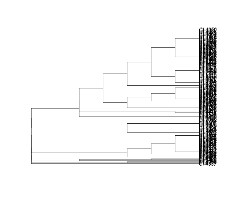
Unfortunately, this tree is ugly and hard to read. We can draw much nicer trees using ggtree. We’ll also read in a metadata file which contains auxiliary information about our isolates.

metadata <- read_csv("metadata.csv")

# We can use %<+% to attach a metadata file to a tree, and the + operator to add
# new layers to our plot

ggtree(mlst_tree, layout = "radial") %<+% metadata + 
  geom_tiplab(size = 2.0) 
  

Now our tree is much more aesthetically pleasing, but more crucially, easier to read.

Is this tree useful, though? Can we learn much about the population structure from it? How does our chosen typing method affect the tree?

Exercise 1 Bonus Work

Try manipulating some of the parameters to ggtree() or geom_tiplab() to produce different visual results. You can view the documentation for these or any other functions either by clicking on it and pressing F1 on your keyboard, or by typing it into the console with a leading ?, e.g. ?ggtree. In the docs for ggtree(), there are some alternative tree layouts you can try.

If you have previous experience with ggplot2, many of the same concepts apply, including the aes() function.

Exercise 2

Your bioinformatician has also provided you with calls core genome multilocus sequence typing scheme (cgMLST). It is structurally similar to classic MLST, however, it uses a much larger number of loci. By having a larger number or loci, more subtle differences between similar strains can be resolved.

Before we continue, we should remember that computers are supposed to make our lives easier and not harder, and with a programming language like R, we can make the computer do as we want. Let’s write a small function that will let us easily reuse the work we did for MLST, but on any similar data.

calculate_tree <- function(calls, pairwise.deletion) {

  tree <-
    calls %>%
    column_to_rownames("genome") %>%
    dist.gene(method = "pairwise", pairwise.deletion = pairwise.deletion) %>%
    hclust() %>%
    as.phylo()

  tree
}

You can use your new function, calculate_tree() to quickly generate and draw a tree for our cgMLST calls.

raw_cgmlst_calls <- read_csv("cgmlst.csv", na="0")

raw_cgmlst_tree <- calculate_tree(raw_cgmlst_calls, pairwise.deletion = FALSE)

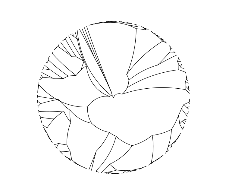
ggtree(raw_cgmlst_tree, layout = "radial")

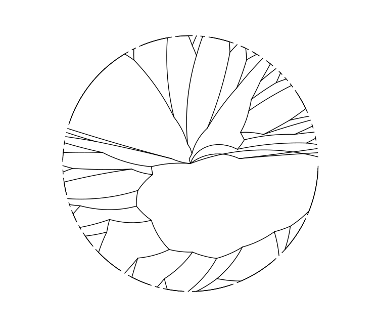
This tree derived from cgMLST allele calls does not look particularly different from the 7-gene MLST tree we drew earlier. What could be affecting this?

One problem that can affect any typing method — but MLST-like methods are particularly sensitive to — is missing data. A locus can be absent because of sequencing error or because that genomic region is not as conserved as was believed. MLST-like methods assume that all loci are always present. In practice due to the size of cgMLST schemes, some tolerance to missing data is required.

Generally, it is preferable to discard poor-quality genomes before removing loci from the scheme. Here, we have encoded missing data as 0 in cgmlst.csv, and told R to treat 0 as absent — NA.

Let’s count the number of missing loci per genome.

missing_per_genome <-
  raw_cgmlst_calls %>%
  rowwise(genome) %>%
  summarize(n_bad = sum(is.na(
    c_across(everything())
    ))
  ) %>%
  arrange(desc(n_bad))

Having calculated the number of missing calls per genome, we can preview the sorted table, look at the summary statistics, and draw a histogram.

missing_per_genome

summary(missing_per_genome$n_bad)

qplot(data=missing_per_genome, x=n_bad, geom="histogram", binwidth=1)

> missing_per_genome
# A tibble: 191 × 2
# Groups:   genome [191]
   genome  n_bad
   <chr>   <int>
 1 CI-5815   242
 2 CI-5603   234
 3 CI-5507   228
 4 CI-5626   227
 5 CI-4990   227
 6 CI-4542    13
 7 CI-4506    12
 8 CI-6226    12
 9 CI-4840    11
10 CI-4995    11
# … with 181 more rows

> summary(missing_per_genome$n_bad)
   Min. 1st Qu.  Median    Mean 3rd Qu.    Max. 
   1.00    5.00    6.00   11.99    8.00  242.00 

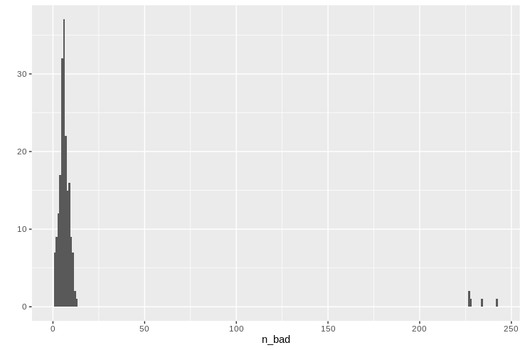
We can can see a normal-ish distribution of missing data around 10 loci per genome, but there are a handful of troublemakers missing almost half of their typing loci. Let’s remember which ones they are so we can later remove them for the greater good of our typing system.

genomes_to_discard <-
  missing_per_genome %>%
  filter(n_bad > 200) %>%
  pull(genome)

We can also look to see if there are any misbehaving loci.

missing_per_locus <-
  raw_cgmlst_calls %>%
  summarise(across(-genome, ~ sum(is.na(.)))) %>%
  pivot_longer(names_to = "locus",
               values_to = "n_bad",
               cols = everything()) %>%
  arrange(desc(n_bad))

We can summarize in a similar manner to the genomes:

missing_per_locus

summary(missing_per_locus$n_bad)

qplot(data = missing_per_locus, x = n_bad, geom = "histogram", binwidth=1)

> missing_per_locus
# A tibble: 595 × 2
   locus       n_bad
   <chr>       <int>
 1 tktA           50
 2 purD           11
 3 group_12331    10
 4 rpmA           10
 5 korB            9
 6 ribA            9
 7 tmk             9
 8 ndhC            9
 9 dnaK            8
10 exoA            8
# … with 584 more rows

> summary(missing_per_locus$n_bad)
   Min. 1st Qu.  Median    Mean 3rd Qu.    Max. 
  0.000   3.000   4.000   3.857   5.000  50.000 

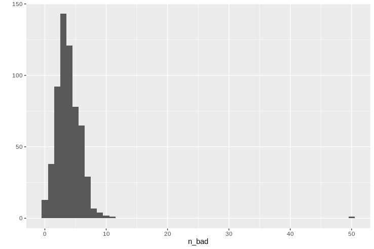
It looks like tktA is particularly troublesome in this population, and so we decide to remove it from the analysis.

We can remove both genomes and locus in a single motion:

filtered_cgmlst_calls <- 
  raw_cgmlst_calls %>%
  filter(!genome %in% genomes_to_discard) %>%
  select(-tktA)

When we calculate the tree, we can also tell ape::dist.gene to, on a pairwise basis, not compare any two genomes at loci they don’t share. This can be done by setting pairwise.deletion=TRUE. If pairwise deletion is FALSE, then any locus missing any calls is dropped from the analysis. This can be an acceptable compromise to make sure the remaining scattered missing loci do not compromise the analysis.

filtered_cgmlst_tree <- calculate_tree(filtered_cgmlst_calls,
                                       pairwise.deletion = TRUE)

ggtree(filtered_cgmlst_tree, layout="radial")

We can see greater discrimination between similar strains now that we have cleaned our data. What would the relative merits have been to not removing missing loci on a pairwise basis?

Exercise 2 Bonus

There is another locus which we may want to discard, albeit not because of missing data. It has another problem. What is it?

Exercise 3

To identify an outbreak within our surveillance data, we need to view the tree in the context of the metadata. We have two variables to look at: the animal from which the isolate was taken and the month when the animal was captured.

We can first save our basic tree visualization, and add metadata annotation to it later.

base_cgmlst_tree <- ggtree(filtered_cgmlst_tree, layout = "circular") 

First we will annotate the tree with information on the host animal.

animal_tree <- 
  base_cgmlst_tree %<+%
  metadata +
  geom_tippoint(aes(colour = animal)) +
  labs(title = "animal")

animal_tree

When can draw a separate tree with the month of capture.

time_tree <-
  base_cgmlst_tree %<+%
  metadata +
  geom_tippoint(aes(colour = date)) +
  labs(title = "Capture Time")
  
time_tree

We can also draw the two trees side-by-side to aid comparison.

plot_list(animal_tree, time_tree,  ncol=2)

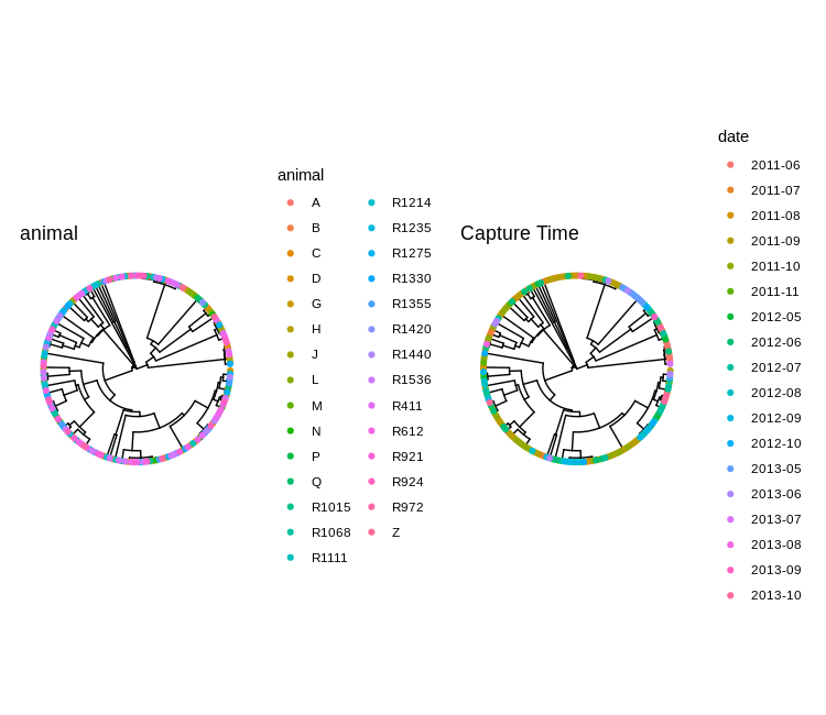
Can you spot the outbreak?

We can narrow the search by highlighting closely-related clusters with several members.

clusters <-
  filtered_cgmlst_tree %>% 
  as.hclust() %>% 
  cutree(h=10) %>% 
  as_tibble(rownames = "genome") %>% 
  rename(cluster = value)

bigger_clusters <-
  clusters %>% 
  group_by(cluster) %>% 
  summarize(n = length(genome)) %>% 
  filter(n >= 6) %>% 
  left_join(clusters) %>% 
  select(genome, cluster)

cluster_mrca_nodes <-
  bigger_clusters %>% 
  group_by(cluster) %>% 
  summarize(cluster_mrca = getMRCA(filtered_cgmlst_tree, genome)) %>% 
  mutate(cluster = factor(cluster))

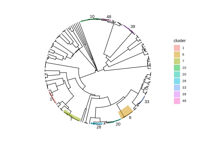
cluster_labelled_tree <-  base_cgmlst_tree + 
  geom_highlight(data=cluster_mrca_nodes, 
                 mapping=aes(node = cluster_mrca,
                             fill = cluster)) +
  geom_cladelab(data=cluster_mrca_nodes,
                mapping=aes(node = cluster_mrca, 
                            label=cluster),
                size=10,
                barsize=0,
                offset=5)

cluster_labelled_tree

Exercise 3 Bonus

Look up the documentation for gheatmap() and see if you can use it as an alternative method for drawing metadata on trees. Although the name implies continuous variables, it can also show discrete variables such as the animal or cluster data.

Exercise 4

We can extract the outbreak cluster for closer inspection via SNP typing methods.

cluster_of_interest <- 39

cluster_genome_names <-
  clusters %>% 
  filter(cluster == cluster_of_interest) %>% 
  select(genome)
  
write_delim(cluster_genome_names, "outbreak_strains.txt", col_names = FALSE)

We’ll use snippy to SNP type the outbreak strains.

In your terminal:

conda activate snippy

mkdir outbreak_strains outbreak_snps

while read strain; do
    ln -sr genomes/$strain.fasta outbreak_strains/$strain.fasta
done < outbreak_strains.txt

for strain in outbreak_strains/*.fasta; do
    name=$(basename $strain .fasta)
    snippy --cpus 4 --outdir outbreak_snps/$name --ref NCTC11168.fasta --ctgs $strain
done

snippy-core outbreak_snps/* --ref NCTC11168.fasta

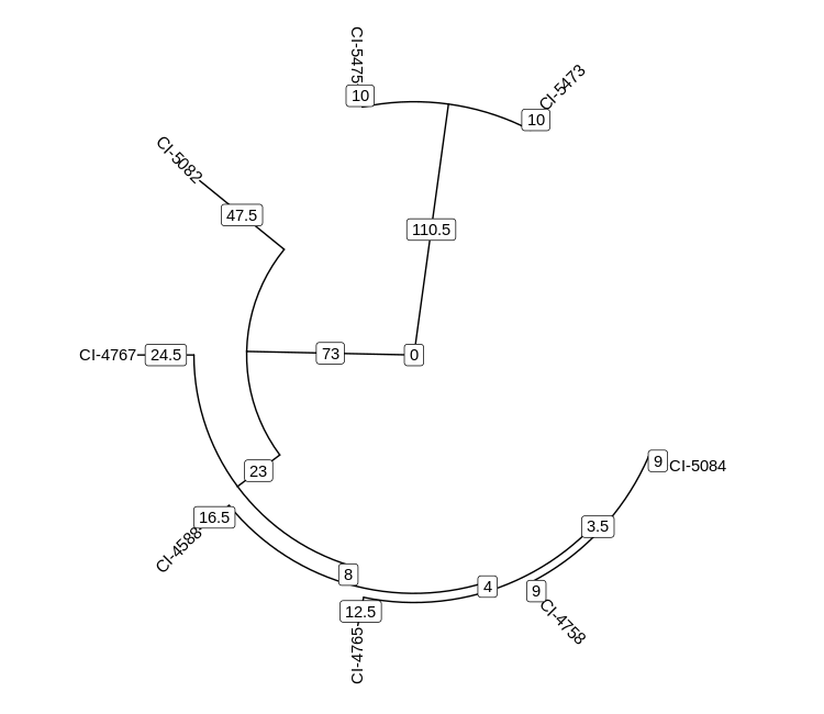
Going back to R, we can load in the Core SNPs, and draw a SNP tree of the outbreak strains.

core_snps <- 
  read_tsv("core.tab") %>% 
  select(-CHR, -REF) %>% 
  pivot_longer(-POS, names_to = "genome") %>% 
  pivot_wider(names_from = "POS") %>% 
  column_to_rownames("genome")

core_snp_tree <- 
  dist.gene(core_snps, method="pairwise") %>%
  hclust() %>% 
  as.phylo()

ggtree(core_snp_tree, layout="circular") %<+% 
  metadata +
  geom_tiplab() +
  geom_label(aes(x = branch, label = branch.length))