IDE Module 4 Lab
Table of contents
1. Introduction
In this tutorial we will be performing phylogenetic and phylodynamic analysis of a set of sequenced SARS-CoV-2 genomes and will be using this information to gain insight into the early introduction of SARS-CoV-2 into Scotland beginning around March 2020. The source of this data is available in the below study:
da Silva Filipe, A., Shepherd, J.G., Williams, T. et al. Genomic epidemiology reveals multiple introductions of SARS-CoV-2 from mainland Europe into Scotland. Nat Microbiol 6, 112–122 (2021). https://doi.org/10.1038/s41564-020-00838-z
We will be referring to this study to compare the phylogenetic trees and other results we generate to the already-published results.
The sequenced genomes from this study are available as part of the COG-UK Consortium and have already been downloaded to your machines.
2. List of software for tutorial
3. Exercise setup
3.1. Copy data files
To begin, we will copy over the necesssary files to ~/workspace.
Commands
cp -r ~/CourseData/IDE_data/module4/ workspace/
cd ~/workspace/module4
When you are finished with these steps you should be inside the directory /home/ubuntu/workspace/module4. You can verify this by running the command pwd.
Output after running pwd
/home/ubuntu/workspace/module4
You should also see a directory data/ in the current directory which contains all the input data. You can verify this by running ls data:
Output after running ls data
MethodsToGetData.md          cog_all.2021-09-27.index  cog_all.index              cog_metadata_2021-09-27.csv.xz  metadata.csv  source_data_fig_1.xlsx
cog_all.2021-09-27.fasta.xz  cog_all.fasta.xz          cog_global_tree.newick.xz  combine-metadata.ipynb          reference
3.2. Activate environment
Next we will activate the conda environment, which will have all the tools needed by this tutorial pre-installed. To do this please run the following:
Commands
conda activate augur
You should see the command-prompt (where you type commands) switch to include (augur) at the beginning, showing you are inside this environment. You should also be able to run the augur command like augur --version and see output:
Output after running augur --version
augur 13.0.0
3.3. Find your IP address
Similar to yesterday, we will want to find the IP address of your machine on AWS so we can access some files from your machine on the web browser. To find your IP address please run:
Commands
curl http://checkip.amazonaws.com
This should print a number like XX.XX.XX.XX. Once you have your address, try going to http://IP-ADDRESS and clicking the link for module4. This page will be referred to later to view some of our output files. In addition, the link precompuated-analysis will contain all the files we will generate during this lab (phylogenetic trees, etc).
4. Building the phylogenetic tree
The overall goal of this lab is to make use of a set of SARS-CoV-2 genomes sequenced and analyzed by the above study to construct our own phylogenetic tree and visualize our epidemiological metadata on top of this tree to gain insight into the early spread of COVID-19 within Scotland. To do this, we will make use of the Augur tool suite, which powers the NextStrain website.
An overview of the basic usage of Augur is as follows (figure from the Augur documentation):

These steps are as follows (we add in an additional visualize step to take a look at some of the output files produced by the Augur pipeline).
- filter: This step extracts a subset of SARS-CoV-2 genomes to be used to build a phylogenetic tree.
- align: This step constructs a multiple sequence alignment from this subset of genomes.
- tree: This step builds a phylogenetic tree, where branch lengths are measured in substitutions/site (a divergence tree).
- (Additional step) visualize: We add this step into the overal Augur pipeline to visualize the constructed tree.
- refine: This step constructs a time tree using our existing tree alongside collection dates of SARS-CoV-2 genomic samples (branch lengths are measured in time).
- export: This step exports the data to be used by Auspice, a version of the visualization system used by NextStrain that lets you examine your own phylogenetic tree and metadata.
Once these steps are completed, we will spend some time comparing the phylogenetic tree and epidemiological metadata to the results published in the existing study.
Step 1: Extract a subset of SARS-CoV-2 genomes (augur filter)
The file data/cog_all.fasta.xz contains all the SARS-CoV-2 genomic sequence data from COG-UK (around 1 million at the end of September 2021). This is much more than what we want to work with. So the first step is to filter the set of genomic samples to only a small subset.
We will use the augur filter command to do this. This command can filter based on a number of criteria, but we will fitler based on matching entries in the metadata.csv file. To do this please run the following:
Commands
# Time: 2 minutes
augur filter --metadata data/metadata.csv --sequences data/cog_all.fasta.xz --sequence-index data/cog_all.index --output filtered.fasta --output-metadata filtered.tsv
You should not expect to see any output from this command until it is finished, which will look like:
Output
1055520 strains were dropped during filtering
        1055520 had no metadata
1324 strains passed all filters
This lets us know that we’ve reduced our dataset from 1 million down to 1324 SARS-CoV-2 genomes, which is a much more managable size.
The output files produced are filtered.fasta and filtered.tsv, which is our reduced sequence data and metadata to be used for later stages. We can use head to get a sense of what’s in these files (head prints only the first 10 lines of a file):
Commands
head filtered.fasta
Output
>Scotland/CVR1222/2020
AGATCTGTTCTCTAAACGAACTTTAAAATCTGTGTGGCTGTCACTCGGCTGCATGCTTAG
TGCACTCACGCAGTATAATTAATAACTAATTACTGTCGTTGACAGGACACGAGTAACTCG
TCTATCTTCTGCAGGCTGCTTACGGTTTCGTCCGTGTTGCAGCCGATCATCAGCACATCT
AGGTTTCGTCCGGGTGTGACCGAAAGGTAAGATGGAGAGCCTTGTCCCTGGTTTCAACGA
GAAAACACACGTCCAACTCAGTTTGCCTGTTTTACAGGTTCGCGACGTGCTCGTACGTGG
CTTTGGAGACTCCGTGGAGGAGGTCTTATCAGAGGCACGTCAACATCTTAAAGATGGCAC
TTGTGGCTTAGTAGAAGTTGAAAAAGGCGTTTTGCCTCAACTTGAACAGCCCTATGTGTT
CATCAAACGTTCGGATGCTCGAACTGCACCTCATGGTCATGTTATGGTTGAGCTGGTAGC
AGAACTCGAAGGCATTCAGTACGGTCGTAGTGGTGAGACACTTGGTGTCCTTGTCCCTCA
Commands
head filtered.tsv | cut -f 1,2 | column -s$'\t' -t
Output
strain                     date
Scotland/CVR380/2020       2020-03-22
Scotland/CVR650/2020       2020-03-25
Scotland/CVR565/2020       2020-03-24
Scotland/EDB194/2020       2020-03-25
Scotland/GCVR-1702C8/2020  2020-03-24
Scotland/GCVR-1709D2/2020  2020-03-25
Scotland/EDB089/2020       2020-03-21
Scotland/GCVR-170E97/2020  2020-03-28
Scotland/EDB193/2020       2020-03-24
For filtered.fasta we can see a portion of the sequence data.
For filtered.tsv, we only select the first two columns (cut -f 1,2) to get just a glimpse of all the metadata in the file. We will use the strain and date columns later to build a time tree (molecular-clock tree). The command column -s$'\t' -t just aligns columns up in our terminal window (using tabs \t as the separator).
Step 2: Construct a multiple sequence alignment of the genomes (augur align)
The next step is to construct a multiple sequence alignment of the genomes, which is required before building a phylogenetic tree. We will be using the command augur align to accomplish this task, but underneath this runs mafft to construct the alignment.
To construct the alignment, please run the following:
Commands
# Time: 7 minutes
augur align --nthreads 4 --sequences filtered.fasta -o alignment.fasta --reference-sequence data/reference/MN908947.fasta
You should expect to see the following:
Output
using mafft to align via:
        mafft --reorder --anysymbol --nomemsave --adjustdirection --thread 4 alignment.fasta.to_align.fasta 1> alignment.fasta 2> alignment.fasta.log

        Katoh et al, Nucleic Acid Research, vol 30, issue 14
        https://doi.org/10.1093%2Fnar%2Fgkf436

[...]

5bp insertion at ref position 11074
        TTT: Scotland/EDB5638/2020, Scotland/GCVR-17028C/2020, Scotland/GCVR-170073/2020, Scotland/GCVR-1717B9/2020
        TTTTT: Scotland/CVR93/2020
1bp insertion at ref position 23903
        WARNING: this insertion was caused due to 'N's or '?'s in provided sequences
1bp insertion at ref position 23958
        WARNING: this insertion was caused due to 'N's or '?'s in provided sequences
Trimmed gaps in MN908947 from the alignment
The meaning of each parameter is as follows:
--nthreads 4: Use 4 threads for the alignment.---sequences filtered.fasta: The input set of sequences in FASTA format.-o alignment.fasta: The output alignment, in FASTA format.--reference-sequence data/reference/MN908947.fasta: The reference genome (the Wuhan-Hu 1 genome). This will be included in our alignment andaugur alignwill, once the alignment is constructed, remove any insertions with respect to this reference genome (useful when identifying and naming specific mutations later on in the augur pipeline).
Once the alignment is complete, you should have a file alignment.fasta in your directory. This is a very similar format as the input file filtered.fasta, but the difference is that sequences have been aligned (possibly by inserting gaps -). This also means that all sequences in alignment.fasta should have the same length (whereas sequences in filtered.fasta, which is not aligned, may have different lengths).
Step 3: Build a Maximum Liklihood phylogenetic tree (augur tree)
The next step is to take the set of aligned genomes alignment.fasta and build a phylogenetic tree (a divergence tree). We will use augur tree for this, but underneath it runs iqtree, which uses the Maximim Likihood method to build a phylogenetic tree. To build a tree, please run the following:
Commands
# Time: 40 seconds
augur tree --nthreads 4 --alignment alignment.fasta -o tree.subs.nwk
You should expect to see the following as output:
Output
Building a tree via:
        iqtree2 -ninit 2 -n 2 -me 0.05 -nt 4 -s alignment-delim.fasta -m GTR  > alignment-delim.iqtree.log
        Nguyen et al: IQ-TREE: A fast and effective stochastic algorithm for estimating maximum likelihood phylogenies.
        Mol. Biol. Evol., 32:268-274. https://doi.org/10.1093/molbev/msu300

[...]

Building original tree took 39.57634449005127 seconds
This produces as output a tree.subs.nwk file, which is the actual phylogenetic tree (in Newick format). You can load this file in a variety of phylogenetic tree viewers (such as http://phylo.io/) but we will further refine this file to work with Auspice.
Another output file is alignment-delim.iqtree.log, which contains additional information from iqtree. You can take a look at this file to get an idea of what iqtree was doing by using tail (prints the last few lines of a file).
Commands
tail -n 20 alignment-delim.fasta.log
Output
Optimal log-likelihood: -51335.133
Rate parameters:  A-C: 0.22548  A-G: 0.93225  A-T: 0.09775  C-G: 0.22911  C-T: 3.62235  G-T: 1.00000
Base frequencies:  A: 0.299  C: 0.184  G: 0.196  T: 0.321
Parameters optimization took 1 rounds (0.932 sec)
BEST SCORE FOUND : -51335.133
Total tree length: 0.034

Total number of iterations: 2
CPU time used for tree search: 41.833 sec (0h:0m:41s)
Wall-clock time used for tree search: 10.602 sec (0h:0m:10s)
Total CPU time used: 132.202 sec (0h:2m:12s)
Total wall-clock time used: 35.790 sec (0h:0m:35s)

Analysis results written to:
  IQ-TREE report:                alignment-delim.fasta.iqtree
  Maximum-likelihood tree:       alignment-delim.fasta.treefile
  Likelihood distances:          alignment-delim.fasta.mldist
  Screen log file:               alignment-delim.fasta.log

Date and Time: Mon Oct  4 23:23:55 2021
As iqtree uses a Maximum Liklihood approach, you will see that it will report the likeihood score of the optimal tree (reported as log-likehoods since likelihood values are very very small).
Note: For this lab we are not looking at branch support values for a tree, but for real-world analysis you may wish to look into including bootstrap support values or approximate likelihood ratio test values. This will give a measure of how well supported each branch in the tree is by the alignment (often as number from 0 for little support to 100 for maximal support). Please see the IQTree documentation for more details.
Step 4: Building a time tree or molecular-clock tree (augur refine)
The tree output by iqtree shows hypothetical evolutionary relationships between different SARS-CoV-2 genomes with branch lengths representing distances between different genomes (in units of substitutions/site or the predicted number of substitutions between genomes divided by the alignment length). However, other methods of measuring distance between genomes are possible. In particular we can incorporate the collection dates of the different SARS-CoV-2 genomes to infer a tree where branches are scaled according to the elapsed time. Such trees are called time trees.
We will use TreeTime to infer a time tree from our phylogenetic tree using collection dates of the SARS-CoV-2 genomes stored in the filtered.tsv metadata file. We will use the augur refine step to run TreeTime and perform some additional refinemint of the tree. To do this, please run the following:
Commands
# Time: 5 minutes
augur refine --alignment alignment.fasta --tree tree.subs.nwk --metadata filtered.tsv --timetree --divergence-units mutations --output-tree tree.time.nwk --output-node-data refine.node.json
You should expect to see the following as output:
Output
augur refine is using TreeTime version 0.8.4

21.73   WARNING: Previous versions of TreeTime (<0.7.0) RECONSTRUCTED sequences of
        tips at positions with AMBIGUOUS bases. This resulted in unexpected
        behavior is some cases and is no longer done by default. If you want to
        replace those ambiguous sites with their most likely state, rerun with
        `reconstruct_tip_states=True` or `--reconstruct-tip-states`.
[...]

Inferred a time resolved phylogeny using TreeTime:
        Sagulenko et al. TreeTime: Maximum-likelihood phylodynamic analysis
        Virus Evolution, vol 4, https://academic.oup.com/ve/article/4/1/vex042/4794731

updated tree written to tree.time.nwk
node attributes written to refine.node.json
The parameters we used are:
--alignment alignment.fasta: The alignment used to build the tree. Used to re-scale the divergence units.--tree tree.subs.nwk: The input tree build using iqtree.--metadata filtered.tsv: The metadata which contains the SARS-CoV-2 genome names (in a column calledstrain) and the sample collection dates (in a column nameddate).--timetree: Build a time tree.--divergence-units mutations: Convert the branch lengths of substitutions/site (mutations/site) to mutations (not needed to build a time tree, this is just used for visualizing the tree later on).--output-tree tree.time.nwk: The output Newick file containing the time tree.--output-node-data refine.node.json: Augur will store additional information here which will let us convert between time trees and substitution trees.
As output, the file tree.time.nwk will contain the time tree while the file refine.node.json contains additional information about the tree. The tree tree.time.nwk will also be rooted based on analysis performed by TreeTime.
Step 5: Package up data for Auspice (augur export)
We will be using Auspice to visualize the tree alongside our metadata. To do this, we need to package up all of the data we have so far into a special file which can be used by Auspice. To do this, please run the following command:
Commands
# Time: 1 second
augur export v2 --tree tree.time.nwk --node-data refine.node.json --title "Example Augur" --output analysis-package.json
You should expect to see the following as output:
Output
WARNING: You didn't provide information on who is maintaining this analysis.

Validating produced JSON
Validating schema of 'analysis-package.json'...
Validating that the JSON is internally consistent...
Validation of 'analysis-package.json' succeeded.
The file analysis-package.json contains both the tree as well as the different branch length units (time and sustitutions) as well as additional data.
5. Visualizing the phylogenetic tree alongside epidemiological metadata
Now that we’ve constructed and packaged up a tree (analysis-package.json), we can visualize this data alongside our metadata (filtered.tsv) using Auspice.
Step 1: Load data into Auspice
To do this, please navigate to http://IP-ADDRESS/module4/analysis/ and download the files analysis-package.json and filtered.tsv to your computer (if the link does not download you can Right-click and select Save link as…).
Next, navigate to https://auspice.us/ and drag the file analysis-package.json onto the page.
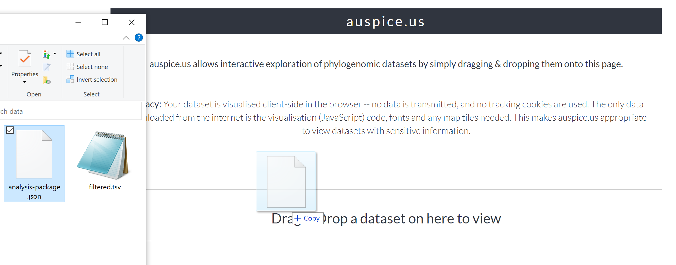
This should result in a phylogenetic tree being loaded that looks like:
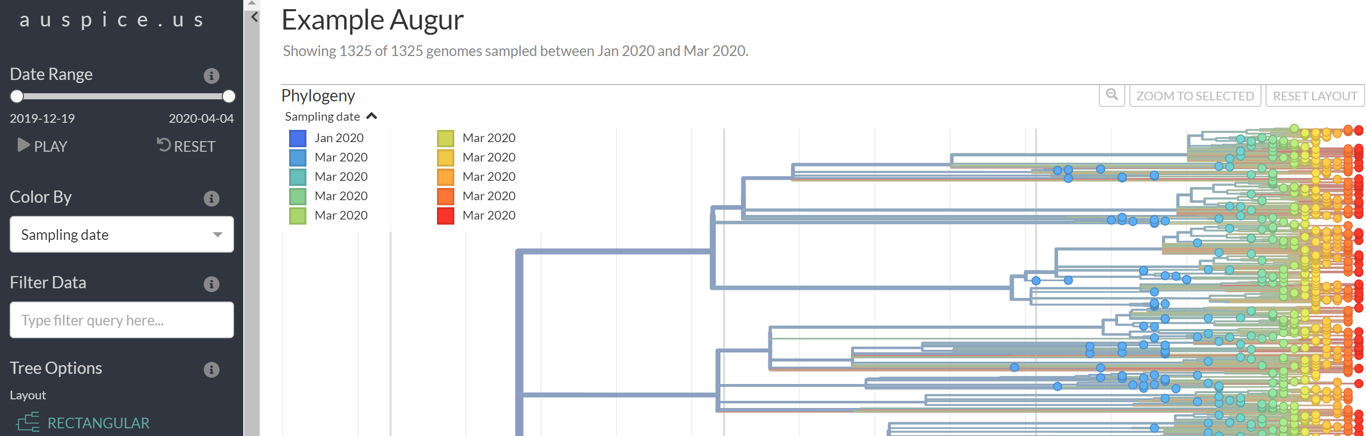
Next, we will load the metadata filtered.tsv file onto this view. To do this, please find and drag-and-drop the filtered.tsv file onto the phylogenetic tree shown in Auspice:
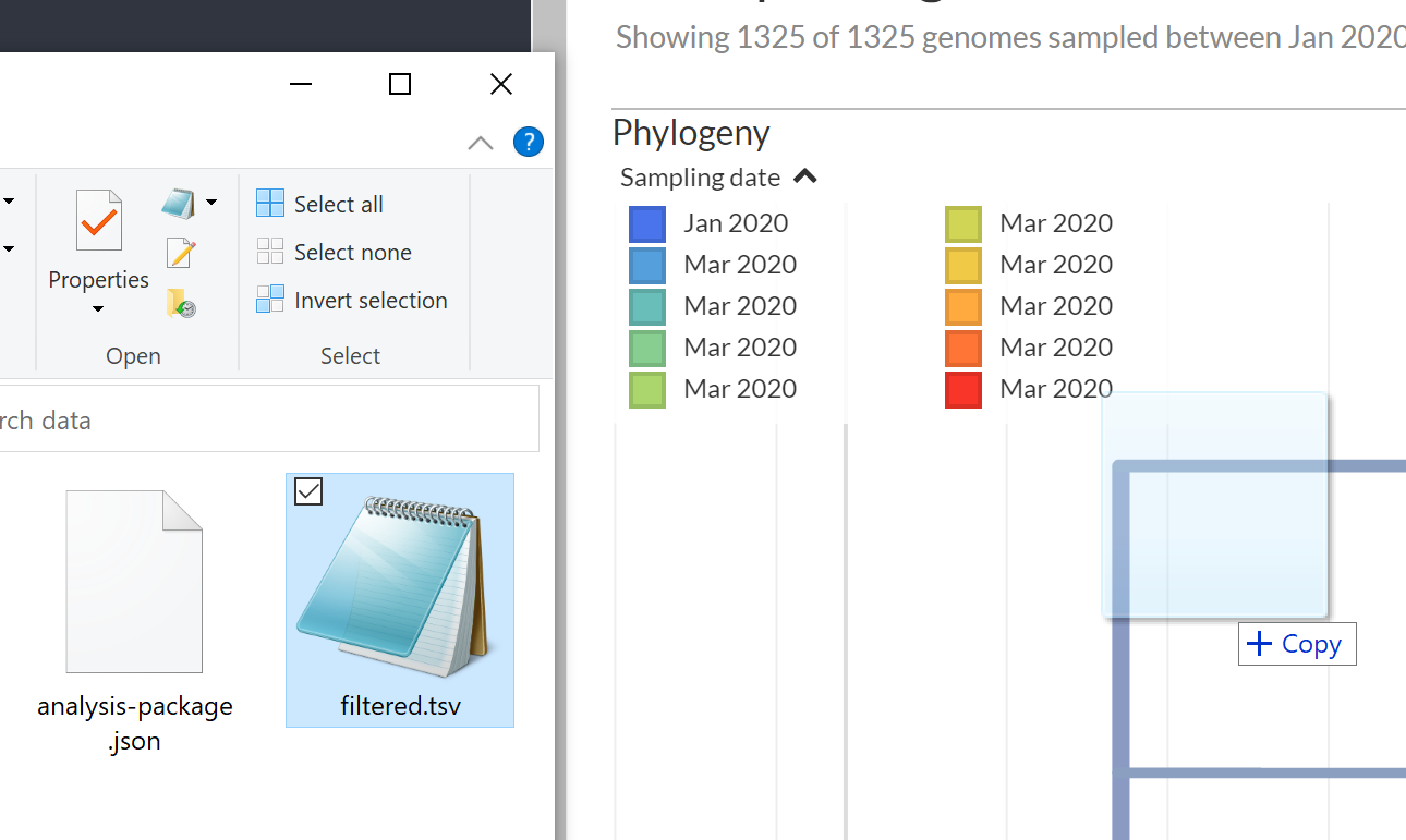
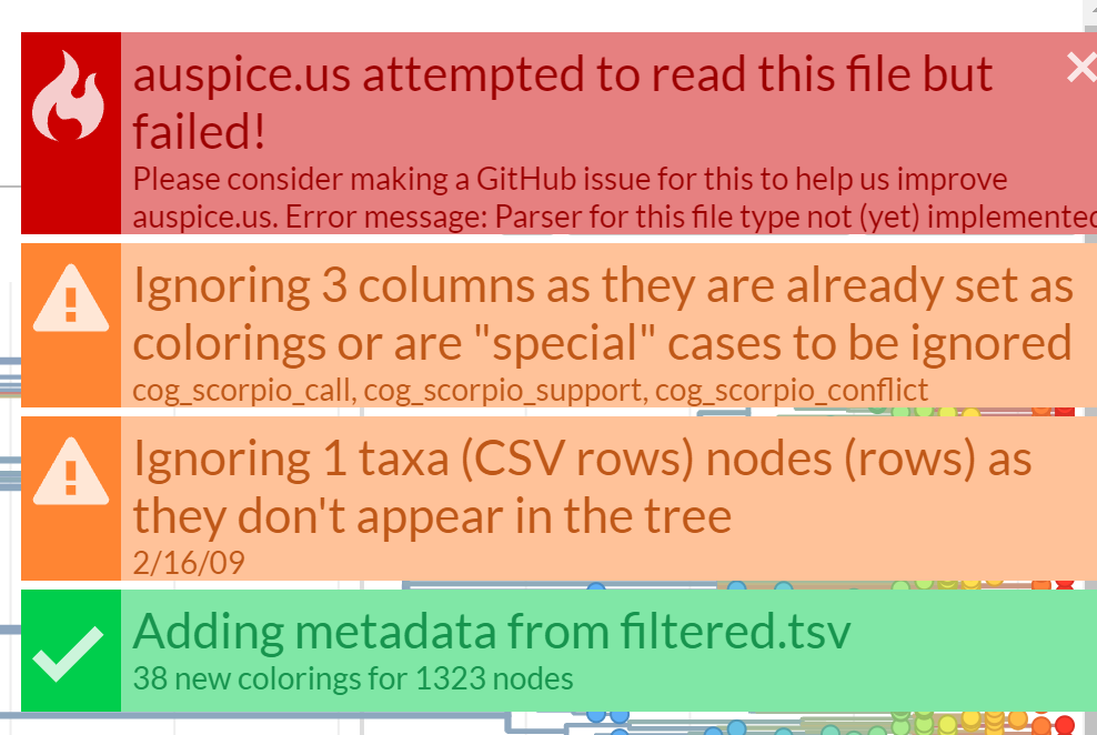
You main get some warning messages showing up, but you should still see a green Added metadata from filtered.tsv message.
Step 2: Explore data
Now you can spend some time to explore the data and get used to the Auspice interface. Try switching between different Tree Layouts, or different Branch Lengths, or colouring the tree by different criteria in the metadata table.
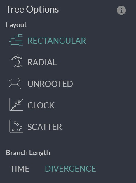
Step 3: Examine particular clades
We are now going to compare the tree we constructed from the tree in Figure 4 of the existing study.
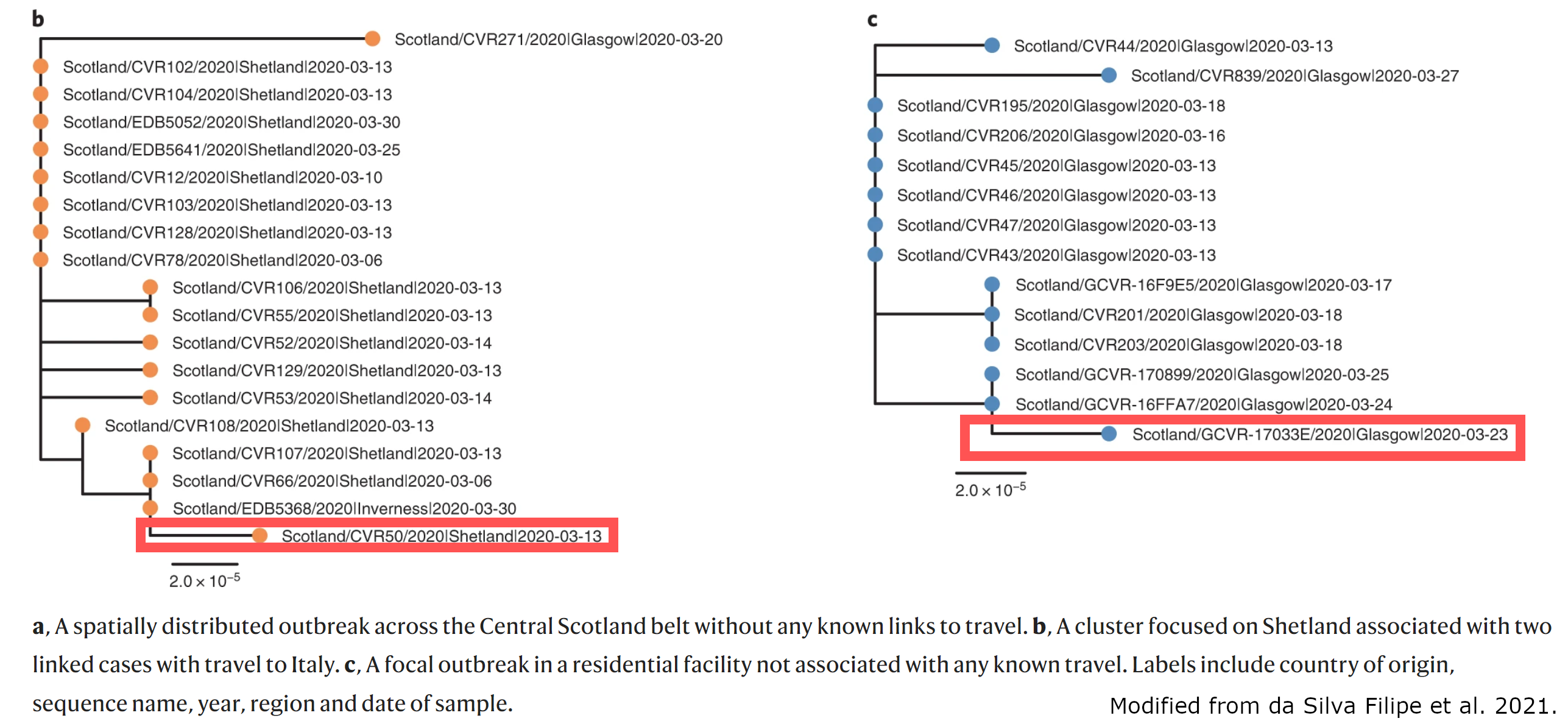
As a first step, let’s examine the tree from Figure 4.b in Auspice. We can do this by searching for one of the genomic samples Scotland/CVR50 in Auspice:
-
Select genome
Scotland/CVR50by using the Filter Data box:
-
Use a combination of Zoom to Selected and the zoom out button (magnifying glass) to show the set of genomic samples around
Scotland/CVR50.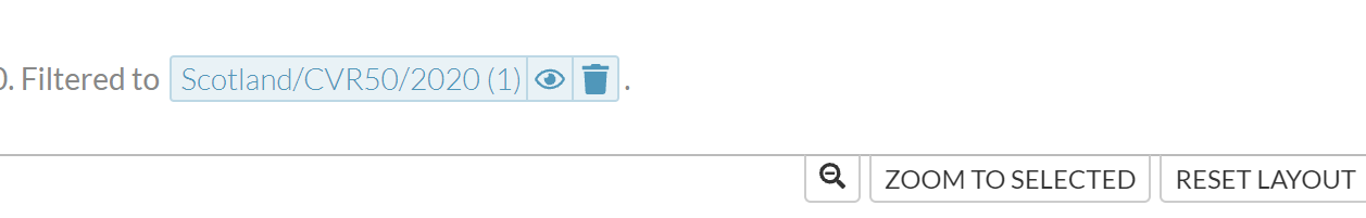
-
Select the Trash icon for the filter to remove it and select to Color by
travel_hx(Travel history). When you are finished you should see something like below.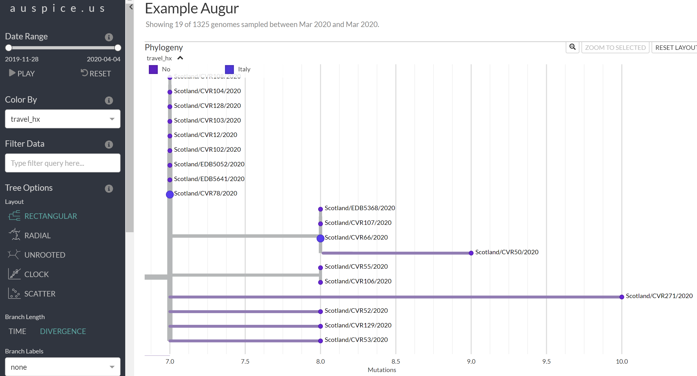
Step 3: Questions
- Compare this tree from that in Figure 4.b above. Are there differences? Is Figure 4.b a Divergence tree or a Time tree?
- Can you spot the two cases associated with travel to Italy in the prior 2 weeks?
- Try out the same procedure for the clade from Figure 4.c (search for
Scotland/GCVR-17033E, you may need to click Reset Layout first). Does it also look simlar to what is shown in Figure 4?
Step 4: Compare predicted dates of common ancestors
Time trees place the leafs of the tree at the collection date for each collected sample and predicts the dates for internal nodes (representing hypothetical ancestors). We can compare our tree (scaled by time) with Figure 5 from the study (an excerpt seen below):
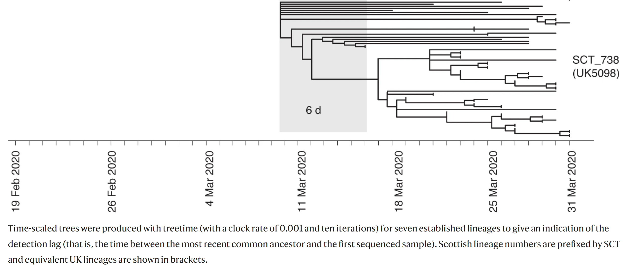
This figure shows a time-scaled tree (dates are shown on the x-axis) and uses this information to infer the detection lag (difference between the time of the common ancestor to this clade and the first sequenced sample).
To compare this figure to our tree, we can search for the listed lineage (UK5098) and zoom into this clade.
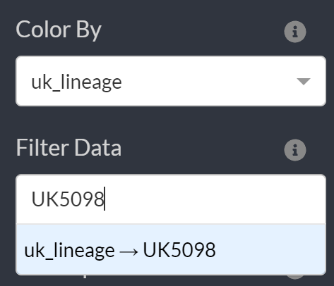
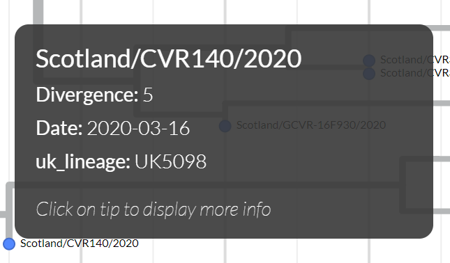
To view sample collection dates you can hover over the particular sample:
Step 4: Questions
- How closely related are some of these genomes in
UK5098(try toggling between Time and Divergence for Branch Length)? - Compare the earliest sample you can find in
UK5098to the predicted date of the most recent common ancestor to all ofUK5098(hover over the branch to get the date). How does this compare to the lag time in Figure 5 above (the shaded gray area that’s labeled6dfor 6 days)?
Note: Our data may not look exactly the same as the figure. We used slightly different software and methods from that of the paper.
6. End of lab
You’ve made it to the end of the lab. Awesome job. If you find you have some extra time, you can explore the data in Auspice further and perhaps compare the tree we have generated to the figures from the study (Figure 4 or Figure 5).
7. Bonus: Visualize tree alongside the alignment
If you have the time, one additional exercise is to look at the phylogenetic tree we have constructed using iqtree alongside the input multiple sequence alignment used to construct the tree. We will be using the ETEToolkit to visualize the tree alongside the alignment. However, the full alignment is quite long, so we will use the BuddySuite set of tools to select only a portion of the alignment to view. To do this please run the following:
Commands
# Make sure you are in the ~/workspace/module4 directory
cd ~/workspace/module4

# Time: 20 seconds
alignbuddy alignment.fasta -er "0:100" > alignment.100.fasta

# Time: 10 seconds
export QT_QPA_PLATFORM="offscreen"
ete3 view -m r -t tree.subs.nwk -i tree.png --alg alignment.100.fasta --alg_type fullseq --alg_format fasta
As output you should expect to see (warnings can be ignored here):
Output
/usr/local/conda/envs/augur/lib/python3.8/site-packages/ete3-3.1.2-py3.7.egg/ete3/evol/parser/codemlparser.py:221: SyntaxWarning: "is" with a literal. Did you mean
"=="?
/usr/local/conda/envs/augur/lib/python3.8/site-packages/ete3-3.1.2-py3.7.egg/ete3/evol/parser/codemlparser.py:221: SyntaxWarning: "is" with a literal. Did you mean
"=="?
Note: alignbuddy produces no output and the warnings produced by ete3 can be ignored.
What these commands do is:
alignbuddy alignment.fasta -er "0:100" > alignment.100.fasta: This extracts the first 100 bp from our multiple sequence alignment and saves to a file alignment.100.fasta.export QT_QPA_PLATFORM="offscreen": This needs to be set before runningete3. This is needed since the machines on AWS don’t have a graphical window system (X Server) attached so we need to tellete3that this is expected (e.g., display is"offscreen").ete3 view ...: This draw the phylogenetic tree (-t tree.subs.nwk) alongside the alignment (--alg alignment.100.fasta) and saves to a a PNG file (-i tree.png). Note: You can save to a PDF file instead by using-i tree.pdf.
Once we have the PNG file saved, you should be able to go to http://IP-ADDRESS/module4/tree.png and view the tree alongside the first 100 bp of the alignment. This will be a pretty big drawing but should look something like:
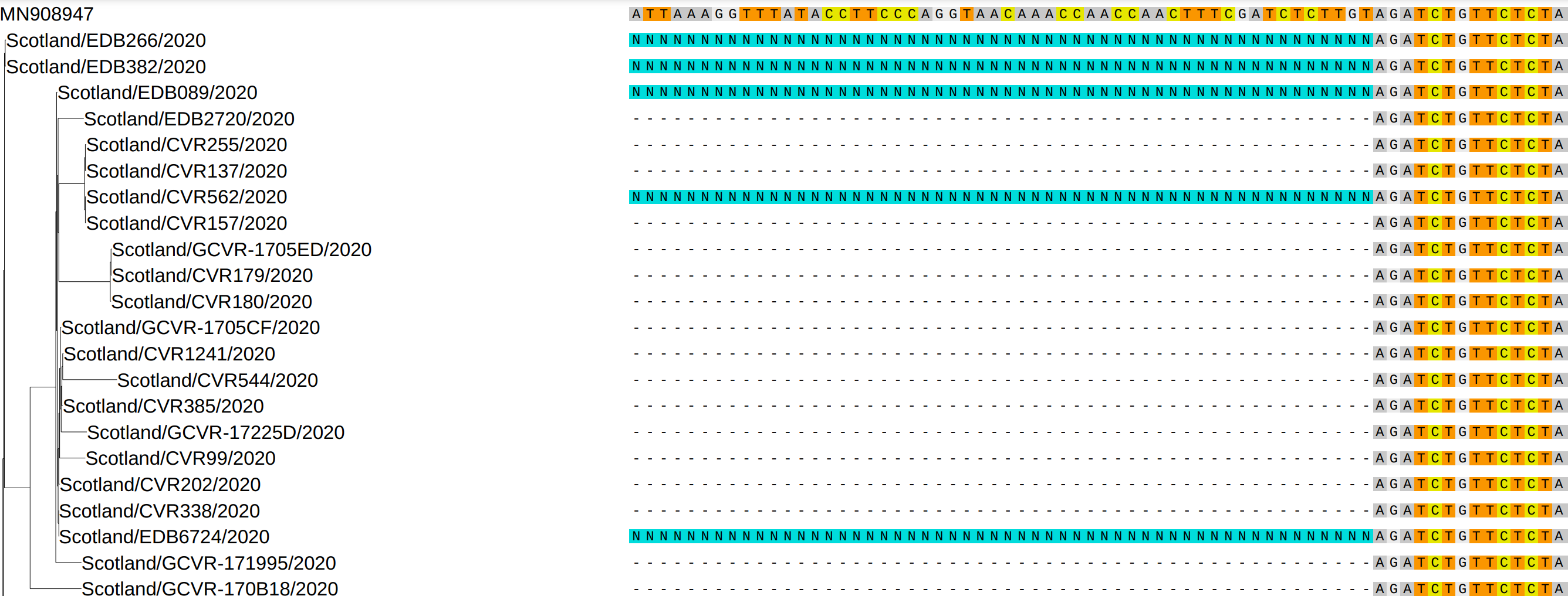
On the right you can see the first 100 bp of the alignment (note that many of the beginning bp are gaps - or ambiguous bases N due to issues with sequencing). On the left you can see the phylogenetic tree. The genome MN908947 is the reference genome which is used as a common coordinate system for naming mutations for SARS-CoV-2.