IDE 2021 Integrated Assignment Answer Key

Developed by: Venus Lau & Jimmy Liu

To start, copy the integrated assignment data directory to your workspace and change your working directory:

cp -r ~/CourseData/IDE_data/integrated_hw/ ~/workspace
cd ~/workspace/integrated_hw

Core genome SNV analysis

Q1: What is the length of the alignment and how is this length determined?

4983515bp. This is the length of the reference genome to which the other genomes were aligned to.

Q2: Which isolate has the most detected variants relative to the reference genome? Which has the least?

SH08-001 had the most detected variant (981 SNVs) while SH12-014 had the least (76 SNVs)

Q3: Which statistics in the variant calling summary file might be useful for identifying outlier (poor quality) samples and why?

The statistics Aligned and Unaligned can provide an indication of reference genome coverage. Including samples with poor reference genome coverage would consequently reduce the length of the overall core genome alignment and decrease the discriminatory power of the cgSNV phylogenetics analysis. The statistic HET indicates the number of heterozygous sites, samples with high HET likely either contain excessive erroneous reads or are contaminated with multiple strains. The statistic LOWCOV indicates the number of sites in the alignment that have low depth of coverage. Variants identified in samples with high LOWCOV have insufficient support/confidence.

Phylogenetic analysis & visualization

Building tree from alignment using FastTree on AWS:

FastTree -nt alignment/heidelberg_core.aln > tree.nwk

Plotting phylogenetic tree in RStudio:

#load packages
library(dplyr)
library(ggtree)
library(ggplot2)

#load files
metadata<-read.csv("metadata.csv")
tree<-read.tree("tree.nwk")

#1. visualize tree, color isolates by isolation date
fig_date<-ggtree(tree, layout="radial") %<+% metadata+
  geom_tiplab(aes(color=as.factor(Isolation_date)) ,size = 2)+ #add labels to tree & colour labels by isolation date
  xlim(0,0.5) + #zoom into the tree
  labs(color="Isolation date")

#save tree to file
ggsave("tree_coloured_by_date.png" , fig_date, width = 6, height = 5, device = "png")

#2. visualize tree, color isolates by isolation source
fig_source<-ggtree(tree, layout="radial") %<+% metadata+
  geom_tiplab(aes(color=as.factor(Source)) ,size = 2)+ #add labels to tree & colour labels by isolation source
  xlim(0,0.5) + #zoom into the tree
  labs(color="Source")

#save tree to file
ggsave("tree_coloured_by_source.png" , fig_source, width = 6, height = 5, device = "png")

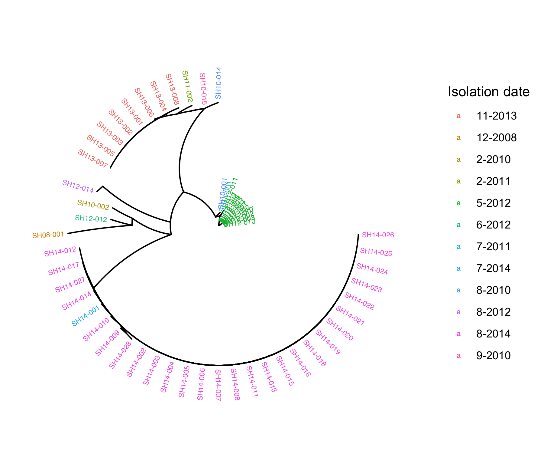
Q4: What does the phylogenetic tree inform you about the relatedness of the isolates within the same outbreak and across different outbreaks?

Isolates of the same outbreak are more phylogenetically related (higher sequence similarity) than isolates collected from different outbreaks

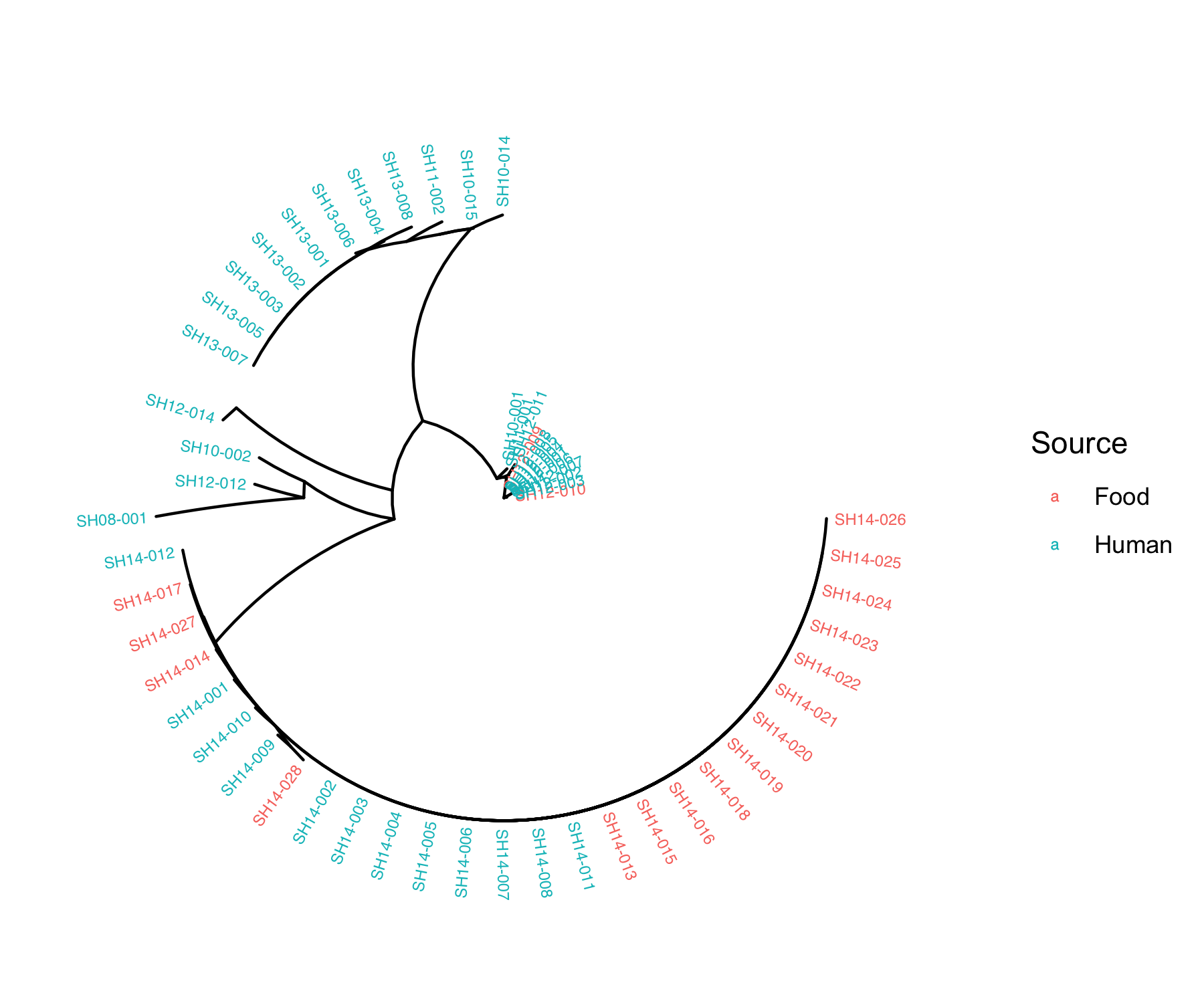
Q5: Do the isolates cluster by isolation source or isolation date?

Isolates tend to cluster by isolation date. ___

Genome Annotation

To search for AMR genes in CARD using ABRicate as example:

# create output directory
mkdir -p abricate/amr
# call abricate
for genome in assemblies/*; do
    abricate --db card assemblies $genome > abricate/amr/$(basename $genome .fa).tab
done
# create a summary file for all genomes
abricate --summary abricate/amr/*.tab > abricate/amr_summary.tab

To visualize the AMR genes summary:

Rscript IDE2021_integrated_hw/abricate_heatmap.R abricate/amr_summary.tab abricate/amr_heatmap.png

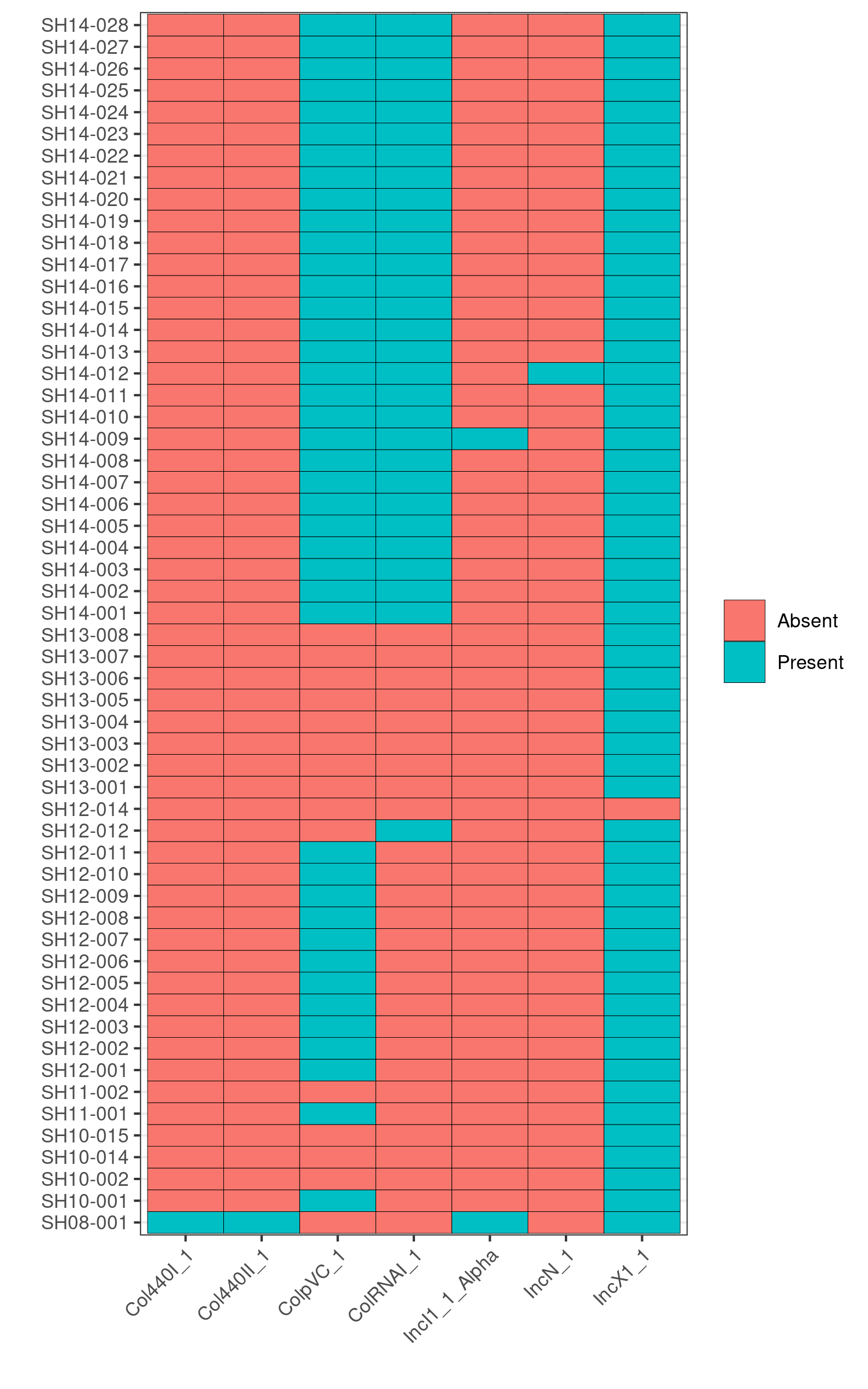
Q6: Can you infer which isolates are epidemiologically linked and which isolates are sporadic cases based on the presence/absence of the plasmids?

Yes, the pattern of presence/absence of plasmids is distinct in each outbreak.

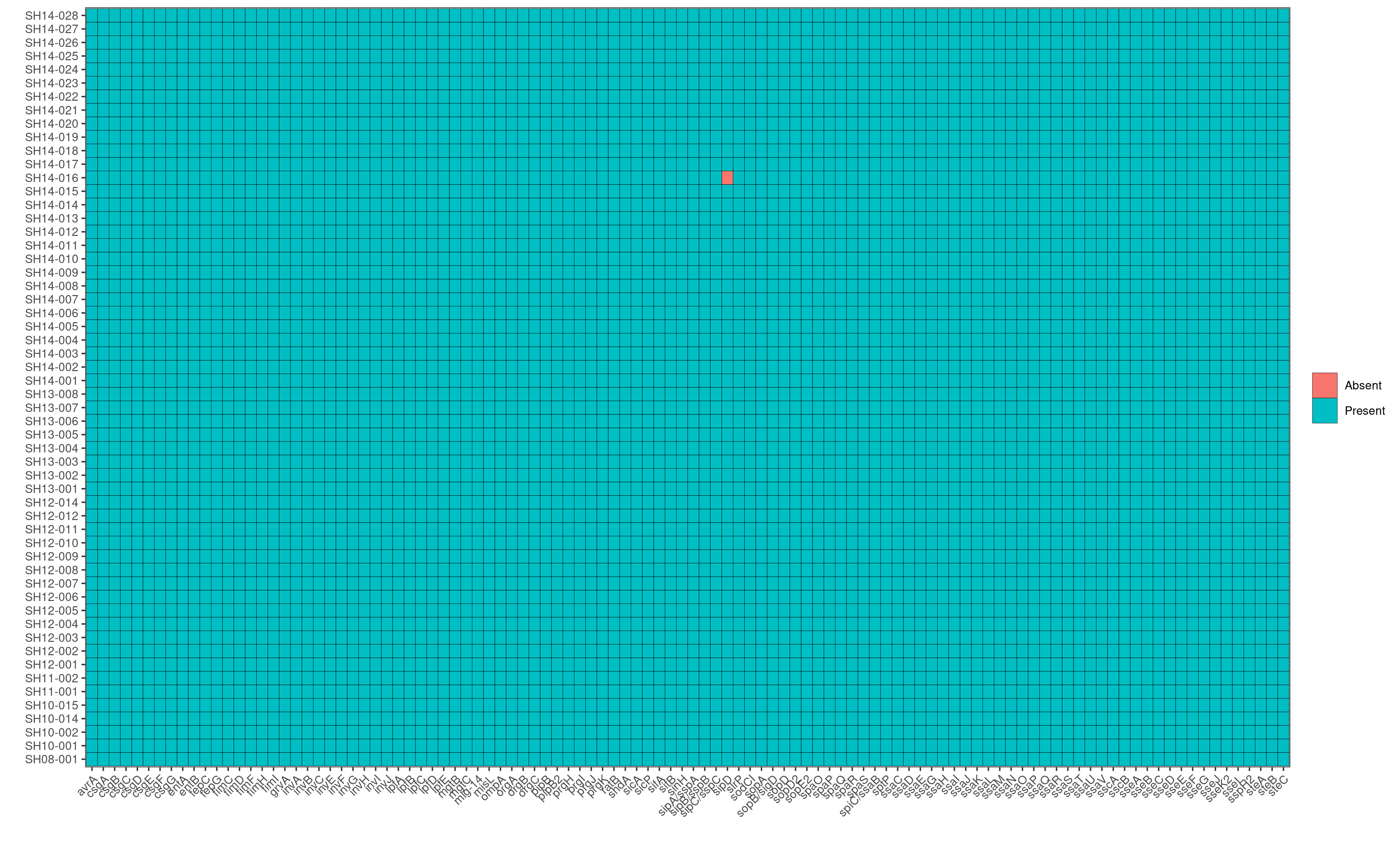
Q7: Do you see the same trend with AMR genes or virulence factors?

No, the majority of isolates, regardless of the outbreak of origin, exhibit the same trend in virulence factors and AMR genes.

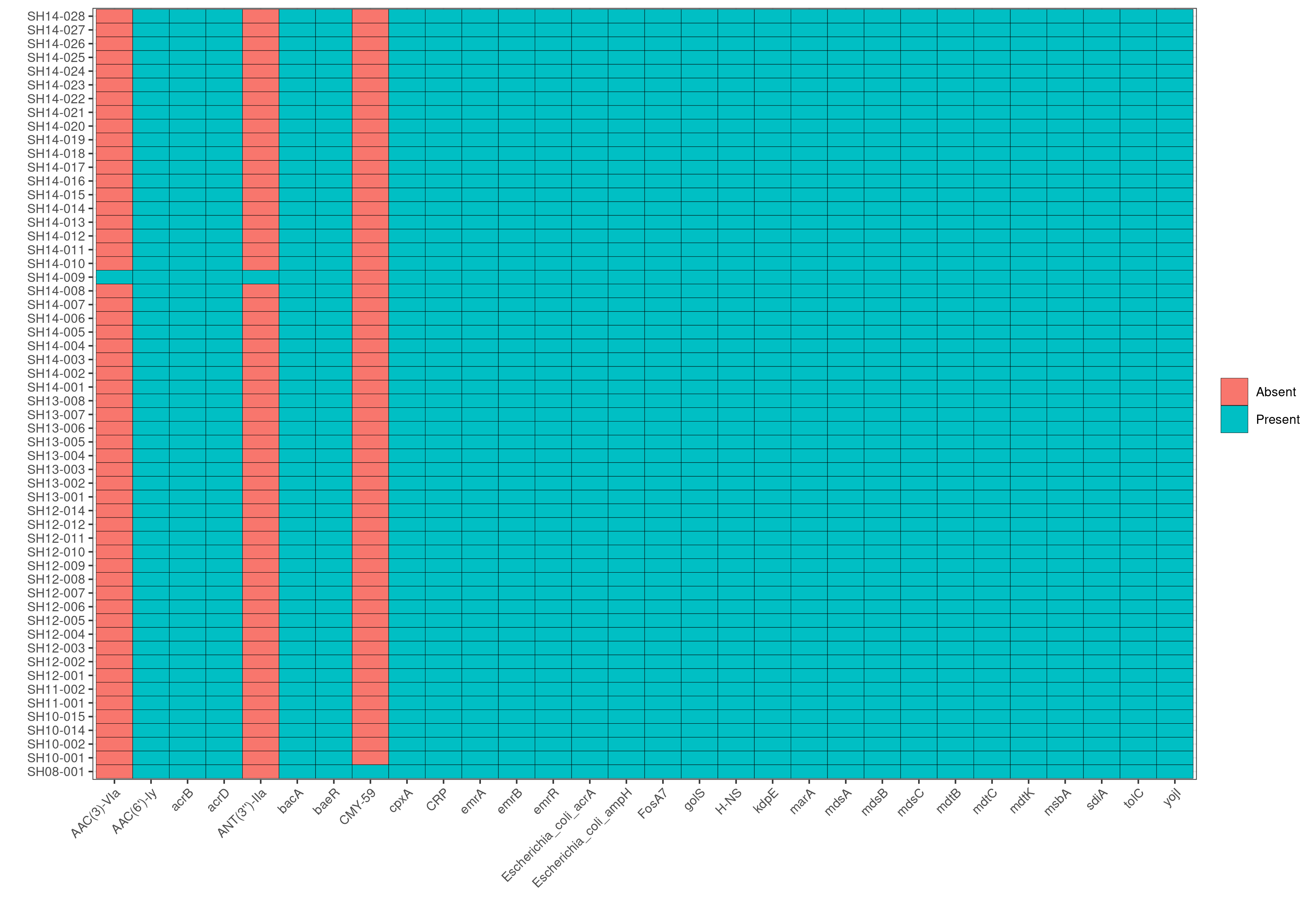
Q8: Looking at the AMR heatmap, which samples likely contain AMR genes encoded on plasmids and how would you verify this looking at ABRicate results?

SH14-009 and SH08-001, because the heatmaps show that they carry 1-2 unique AMR genes that are not present in any other genomes in the dataset. Furthermore, in the plasmids heatmap, we also observe that SH14-009 and SH08-001 carry unique plasmids; hence the unqiue AMR genes are most likely encoded by these unique plasmids.

To verify this, we first identify the contig name associated with the unique plasmids from the invidiual abricate results. For example, based on the plasmids heatmap, we observe that SH14-009 carries the unique plasmid, IncI1_1_Alpha.

Running: grep IncI_1_Alpha abricate/plasmids/SH14-009.tab, we find that the unique plasmid is associated with the contig name, CP016585.1

Subsequently, we can search in the AMR results of SH14-009 to identify AMR genes that are present in the contig CP016585.1 by running grep CP016585.1 abricate/amr/SH14-009.tab. And indeed, we find that the contig contains two AMR genes: AAC(3)-VIa and ANT(3’’)-IIa, which in fact are the two AMR genes unique to SH14-009!

Q9: Aside from plasmids, AMR genes and VF, can you think of other genetic features in bacterial genomes that may help discriminate between these outbreaks?

CRISPR arrays, insertional elements, genomic Islands, phage elements, integrative conjugative elements