Infectious Disease Genomic Epidemiology Module 8 Lab
Table of contents
- Introduction
- Software
- Setup
- Exercise
- Final words
1. Introduction
This tutorial aims to introduce a variety of software and concepts related to detecting emerging pathogens from a complex host sample. The provided data and methods are derived from real-world data, but have been modified to either illustrate a specific learning objective or to reduce the complexity of the problem. Contamination and a lack of large and accurate databases render detection of microbial pathogens difficult. As a disclaimer, all results produced from the tools described in this tutorial and others must also be verified with supplementary bioinformatics or wet-laboratory techniques.
2. List of software for tutorial and its respective documentation
The workshop machines already have this software installed within a conda environment, but to perform this analysis later on, you can make use of the conda environment located at environment.yml to install the necessary software.
3. Exercise setup
3.1. Copy data files
To begin, we will copy over the exercises to ~/workspace. This let’s use view the resulting output files in a web browser.
Commands
cp -r ~/CourseData/IDE_data/module8/module8_workspace/ ~/workspace/
cd ~/workspace/module8_workspace/analysis
When you are finished with these steps you should be inside the directory /home/ubuntu/workspace/module8_workspace/analysis. You can verify this by running the command pwd.
Output after running pwd
/home/ubuntu/workspace/module8_workspace/analysis
You should also have a directory like data/ one directory up from here. To check this, you can run ls ../:
Output after running ls ../
analysis data precomputed-analysis
3.2. Activate environment
Next we will activate the conda environment, which will have all the tools needed by this tutorial pre-installed. To do this please run the following:
Commands
conda activate module8-emerging-pathogen
You should see the command-prompt (where you type commands) switch to include (module8-emerging-pathogen) at the beginning, showing you are inside this environment. You should also be able to run one of the commands like kraken2 --version and see output:
Output after running kraken2 --version
Kraken version 2.1.2
Copyright 2013-2021, Derrick Wood (dwood@cs.jhu.edu)
3.3. Verify your workshop machine URL
This exercise will produce output files intended to be viewed in a web browser. These should be accessible by going to http://xx.uhn-hpc.ca in your web browser where xx is your particular number (like 01, 02, etc). If you are able to view a list of files and directories, try clicking the link for module8_workspace. This page will be referred to later to view some of our output files. In addition, the link precompuated-analysis will contain all the files we will generate during this lab.
4. Exercise
4.1. Patient Background:
A 41-year-old man was admitted to a hospital 6 days after the onset of disease. He reported fever, chest tightness, unproductive cough, pain and weakness. Preliminary investigations excluded the presence of influenza virus, Chlamydia pneumoniae, Mycoplasma pneumoniae, and other common respiratory pathogens. After 3 days of treatment the patient was admitted to the intensive care unit, and 6 days following admission the patient was transferred to another hospital.
To further investigate the cause of illness, a sample of bronchoalveolar lavage fluid (BALF) was collected from the patient and metatranscriptomic sequencing was performed (that is, the RNA from the sample was sequenced). In this lab, you will examine the metatranscriptomic data using a number of bioinformatics methods and tools to attempt to identify the cause of the illness.
Note: The patient information and data was derived from a real study (shown at the end of the lab).
4.2. Overview
We will proceed through the following steps to attempt to diagnose the situation.
- Trim and clean sequence reads using
fastp - Filter host (human) reads with
kat - Run Kraken2 with a bacterial and viral database to look at the taxonomic makeup of the reads.
- Assemble the metatranscriptome with
megahit - Examine assembly quality using
quastand possible pathogens withblast
Assembly-free approach
The first set of steps follows through an assembly-free approach where we will perform taxonomic classification of the reads without constructing a metagenomics assembly.
Step 1: Examine the reads
Let’s first take a moment to examine the reads from the metatranscrimptomic sequencing. Note that for metatranscriptomic sequencing, while we are sequencing the RNA, this was performed by first generating complementary DNA (cDNA) to the RNA and sequencing the cDNA. Hence you will see thymine (T) instead of uracil (U) in the sequence data.
The reads were generated from paired-end sequencing, which means that a particular fragment (of cDNA) was sequenced twice–once from either end (see the Illumina Paired vs. Single-End Reads for some additional details). These pairs of cDNA sequence reads are stored as separate files (named emerging-pathogen-reads_1.fastq.gz and emerging-pathogen-reads_2.fastq.gz). You can see each file by running ls:
Commands
ls ../data
Output
emerging-pathogen-reads_1.fastq.gz emerging-pathogen-reads_2.fastq.gz
We can look at the contents of one of the files by running less (you can look at the other pair of reads too, but it will look very similar):
Commands
less ../data/emerging-pathogen-reads_1.fastq.gz
Output
@SRR10971381.5 5 length=151
NNNNNNNNNNNNNNNNNNNNNNNNNNNNNNNNNNNNNNNNNNNNNNNNNNNNNNNNNNNNNNNNNNNNNNNNNNNNNNNNNNNNNNNNNNNNNNNNNNNNNNNNNNNNNNNNNNNNNNNNNNNNNNNNNNNNNNNNNNNNNNNNNNNNNNN
+
!!!!!!!!!!!!!!!!!!!!!!!!!!!!!!!!!!!!!!!!!!!!!!!!!!!!!!!!!!!!!!!!!!!!!!!!!!!!!!!!!!!!!!!!!!!!!!!!!!!!!!!!!!!!!!!!!!!!!!!!!!!!!!!!!!!!!!!!!!!!!!!!!!!!!!!
@SRR10971381.7 7 length=151
NNNNNNNNNNNNNNNNNNNNNNNNNNNNNNNNNNNNNNNNNNNNNNNNNNNNNNNNNNNNNNNNNNNNNNNNNNNNNNNNNNNNNNNNNNNNNNNNNNNNNNNNNNNNNNNNNNNNNNNNNNNNNNNNNNNNNNNNNNNNNNNNNNNNNNN
+
!!!!!!!!!!!!!!!!!!!!!!!!!!!!!!!!!!!!!!!!!!!!!!!!!!!!!!!!!!!!!!!!!!!!!!!!!!!!!!!!!!!!!!!!!!!!!!!!!!!!!!!!!!!!!!!!!!!!!!!!!!!!!!!!!!!!!!!!!!!!!!!!!!!!!!!
@SRR10971381.33 33 length=115
NNNNNNNNNNNNNNNNNNNNNNNNNNNNNNNNNNNNNNNNNNNNNNNNNNNNNNNNNNNNNNNNNNNNNNNNNNNNNNNNNNNNNNNNNNNNNNNNNNNNNNNNNNNNNNNNNNN
+
!!!!!!!!!!!!!!!!!!!!!!!!!!!!!!!!!!!!!!!!!!!!!!!!!!!!!!!!!!!!!!!!!!!!!!!!!!!!!!!!!!!!!!!!!!!!!!!!!!!!!!!!!!!!!!!!!!!
@SRR10971381.56 56 length=151
CCCGTGTTCGATTGGCATTTCACCCCTATCCACAACTCATCCCAAAGCTTTTCAACGCTCACGAGTTCGGTCCTCCACACAATTTTACCTGTGCTTCAACCTGGCCATGGATAGATCACTACGGTTTCGGGTCTACTATTACTAACTGAAC
+
FFFFFFFAFFFFFFAFFFFFF6FFFFFFFFF/FFFFFFFFFFFF/FFFFFFFFFFFFFFFFFAFFFFFFFFFFFAFFFFF/FFAF/FAFFFFFFFFFAFFFF/FFFFFFFFFFF/F=FF/FFFFA6FAFFFFF//FFAFFFFFFAFFFFFF
These reads are in the FASTQ, which stores a single read as a block of 4 lines: identifier, sequence, + (separator), quality scores. In this file, we can see a lot of lines with NNN... for the sequence letters, which means that these portions of the read are not determined. We will remove some of these undetermined (and uninformative) reads in the next step.
Step 2: Clean and examine quality of the reads
As we saw from looking at the data, reads that come directly off of a sequencer may be of variable quality which might impact the downstream analysis. We will use the software fastp to both clean and trim reads (removing poor-quality reads or sequencing adapters) as well as examine the quality of the reads. To do this please run the following (the expected time of this command is shown as # Time: 30 seconds).
Commands
# Time: 30 seconds
fastp --detect_adapter_for_pe --in1 ../data/emerging-pathogen-reads_1.fastq.gz --in2 ../data/emerging-pathogen-reads_2.fastq.gz --out1 cleaned_1.fastq --out2 cleaned_2.fastq
You should see the following as output:
Output
Detecting adapter sequence for read1...
No adapter detected for read1

Detecting adapter sequence for read2...
No adapter detected for read2
[...]
Insert size peak (evaluated by paired-end reads): 150

JSON report: fastp.json
HTML report: fastp.html

fastp --detect_adapter_for_pe --in1 ../data/emerging-pathogen-reads_1.fastq.gz --in2 ../data/emerging-pathogen-reads_2.fastq.gz --out1 cleaned_1.fastq --out2 cleaned_2.fastq
fastp v0.23.2, time used: 22 seconds
Examine output
You should now be able to nagivate to < http://xx.uhn-hpc.ca/module8_workspace/analysis> and see some of the output files. In particular, you should be able to find fastp.html, which contains a report of the quality of the reads and how many were removed. Please take a look at this report now:
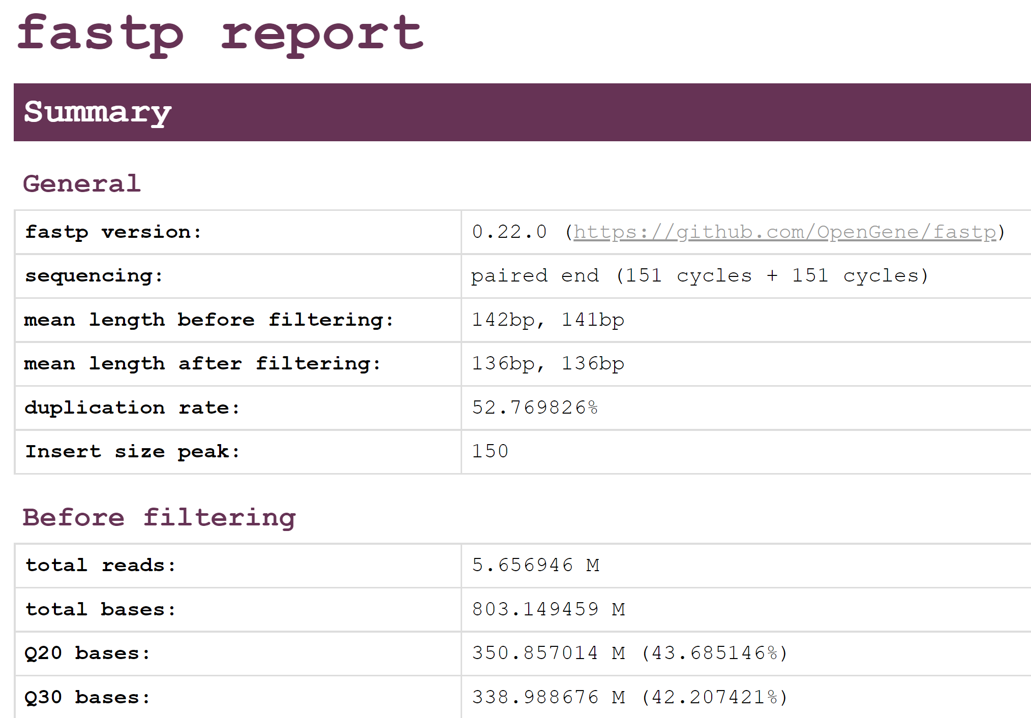
This should show an overview of the quality of the reads before and after filtering with fastp. Using this report, please answer the following questions.
Step 2: Questions
- Looking at the Filtering result section, how many reads passed filters? How many were removed due to low quality? How many were removed due to too many N?
- Looking at the Adapters section, were there many adapters that needed to be trimmed in this data?
- Compare the quality and base contents plots Before filtering and After filtering? How do they differ?
Step 3: Host read filtering
The next step is to remove any host reads (in this case Human reads) from our dataset as we are not focused on examining host reads. There are several different tools that can be used to filter out host reads such as Bowtie2 or KAT. In this demonstration, we have selected to run KAT followed by Kraken2, but you could likely accomplish something similar by using Bowtie2 followed by Kraken2.
Command documentation is available here
KAT works by breaking down each read into small fragements of length k, k-mers, and compares them to a k-mer database of the human reference genome. Subsequently, the complete read is either assigned into a matched or unmatched (filtered) file if 10% of the k-mers in the read have been found in the human database.
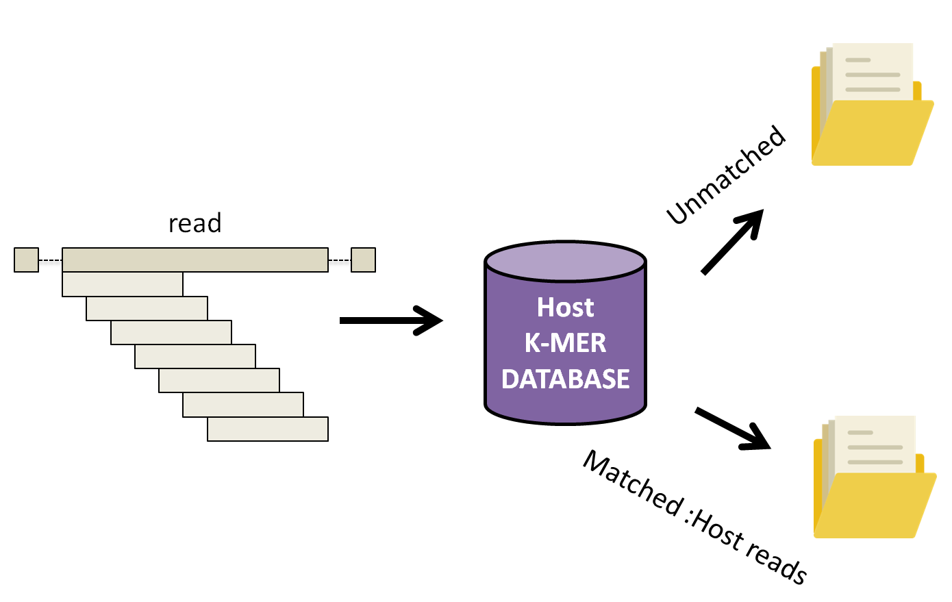
Let’s run KAT now.
Commands
# Time: 3 minutes
kat filter seq -t 4 -i -o filtered --seq cleaned_1.fastq --seq2 cleaned_2.fastq ~/CourseData/IDE_data/module8/db/kat_db/human_kmers.jf
The arguments for this command are:
filter seq: Specifies that we are running a specific subcommand to filter sequences.-t 4: The number of threads to use (we have 4 CPU cores on these machines so we are using 4 threads).--seq --seq2arguments to provide corresponding forward and reverse fastq reads (the cleaned reads fromfastp)-i: Inverts the filter, that is we wish to output sequences not found in the human kmer database to a file.-o filteredProvide prefix for all files generated by the command. In our case, we will have two output files filtered.in.R1.fastq and filetered.in.R2.fastq.~/CourseData/IDE_data/module8/db/kat_db/human_kmers.jfthe human k-mer database
As the command is running you should see the following output on your screen:
Output
Kmer Analysis Toolkit (KAT) V2.4.2

Running KAT in filter sequence mode
-----------------------------------

Loading hashes into memory... done.  Time taken: 40.7s

Filtering sequences ...
Processed 100000 pairs
Processed 200000 pairs
[...]
Finished filtering.  Time taken: 130.5s

Found 1127908 / 1306231 to keep

KAT filter seq completed.
Total runtime: 182.8s
If the command was successful, your current directory should contain two new files:
filtered.in.R1.fastqfiltered.in.R2.fastq
These are the set of reads minus any reads that matched the human genome. The message Found 1127908 / 1306231 to keep tells us how many read-pairs were kept (the number in the filtered.in.*.fastq files) vs. the total number of read-pairs.
Step 4: Classify reads using Kraken2 database
Now that we have most, if not all, host reads filtered out, it’s time to classify the remaining reads to identify the likely taxonomic category they belong to.
Database selection is one of the most crucial parts of running Kraken. One of the many factors that must be considered is the computational resources available. Our current AWS image for the course has only 16G of memory. A major disadvantage of Kraken2 is that it loads the entire database into memory. With the standard viral, bacterial, and archael database on the order of 50 GB we would be unable to run the full database on the course machine. To help mitigate this, Kraken2 allows reduced databases to be constructed, which will still give reasonable results. We have constructed our own smaller Kraken2 database using only bacterial, human, and viral data. We will be using this database.
Lets run the following command in our current directory to classify our reads against the Kraken2 database.
Commands
# Time: 1 minute
kraken2 --db ~/CourseData/IDE_data/module8/db/kraken2_db --threads 4 --paired --output kraken_out.txt --report kraken_report.txt --unclassified-out kraken2_unclassified#.fastq filtered.in.R1.fastq filtered.in.R2.fastq
This should produce output similar to below:
Output
Loading database information... done.
1127908 sequences (315.54 Mbp) processed in 7.344s (9214.6 Kseq/m, 2577.83 Mbp/m).
  880599 sequences classified (78.07%)
  247309 sequences unclassified (21.93%)
Examine kraken_report.txt
Let’s examine the text-based report of Kraken2:
Commands
less kraken_report.txt
This should produce output similar to the following:
 21.93  247309  247309  U       0       unclassified
 78.07  880599  30      R       1       root
 78.01  879899  124     R1      131567    cellular organisms
 76.37  861411  19285   D       2           Bacteria
 56.53  637572  2       D1      1783270       FCB group
 56.53  637558  1571    D2      68336           Bacteroidetes/Chlorobi group
 56.39  635982  1901    P       976               Bacteroidetes
 55.10  621496  35      C       200643              Bacteroidia
 55.09  621417  19584   O       171549                Bacteroidales
 53.18  599872  2464    F       171552                  Prevotellaceae
 52.96  597396  397538  G       838                       Prevotella
  4.74  53473   53473   S       28137                       Prevotella veroralis
[...]
This will show the top taxonomic ranks (right-most column) as well as the percent and number of reads that fall into these categories (left-most columns). For example:
- The very first row
21.93 247309 247309 U 0 unclassifiedshows us that 247309 (21.93%) of the reads processed by Kraken2 are unclassified (remember we only used a database containing bacterial, viral, and human representatives). - The 4th line
76.37 861411 19285 D 2 Bacteriatells us that 861411 (76.37%) of our reads fall into the Bacteria domain (theDin the fourth column is the taxonomic rank,Domain). The number19285tells us that19285of the reads are assigned directly to the Bacteria domain but cannot be assigned to any lower taxonomic rank (they match with too many diverse types of bacteria).
More details about how to read this report can be found at https://github.com/DerrickWood/kraken2/wiki/Manual#sample-report-output-format. In the next step we will represent this data visually as a multi-layered pie chart.
Examine kraken_out.txt
Let’s also take a look at kraken_out.txt. This file contains the kraken2 results, but divided up into a classification for every read.
Commands
column -s$'\t' -t kraken_out.txt | less -S
column formats a text file (kraken_out.txt) into multiple columns according to a tab delimiter character (flag -s'$\t') and produces a table (flag -t).
Output
C       SRR10971381.56  29465   151|151 0:40 909932:2 0:8 909932:2 0:20 29465:4 0:7 178327>
C       SRR10971381.97  838     122|122 0:44 2:5 0:23 838:1 0:10 838:2 0:3 |:| 0:3 838:2 0>
C       SRR10971381.126 9606    109|109 0:2 9606:5 0:7 9606:1 0:12 9606:1 0:47 |:| 0:47 96>
C       SRR10971381.135 838     151|151 0:95 838:3 0:19 |:| 0:15 838:1 0:12 838:5 0:6 838:>
C       SRR10971381.219 1177574 151|151 0:11 838:3 0:5 838:2 0:9 838:5 0:11 838:1 976:5 83>
C       SRR10971381.223 838     151|151 0:117 |:| 0:61 838:4 0:40 838:1 0:11
[...]
This shows us a taxonomic classification for every read (one read per line). For example:
- On the first line,
C SRR10971381.56 29465tells us that this read with identifierSRR10971381.56is classifiedC(matches to something in the Kraken2 database) and matches to the taxonomic category29465, which is the NCBI taxonomy identifer. In this case29465corresponds to Veillonella.
More information on interpreting this file can be found at https://github.com/DerrickWood/kraken2/wiki/Manual#standard-kraken-output-format.
Step 5: Generate an interactive html-based report using Pavian
Instead of reading text-based files like above, we can visualize this information using Pavian, which can be used to construct an interactive summary and visualization of metagenomics data. Pavian supports a number of metagenomics analysis software outputs, including Kraken/Kraken2. To visualize the Kraken2 output we just generated, we can upload the kraken_report.txt file to the web application. Please do this now using the following steps:
- Download the
kraken_report.txtto your local machine from http://xx.uhn-hpc.ca/module8_workspace/analysis (you can right-click and select Save as… on the file). -
Visit the Pavian website and click on Upload files > Browse… and select the file
kraken_report.txtwe just downloaded.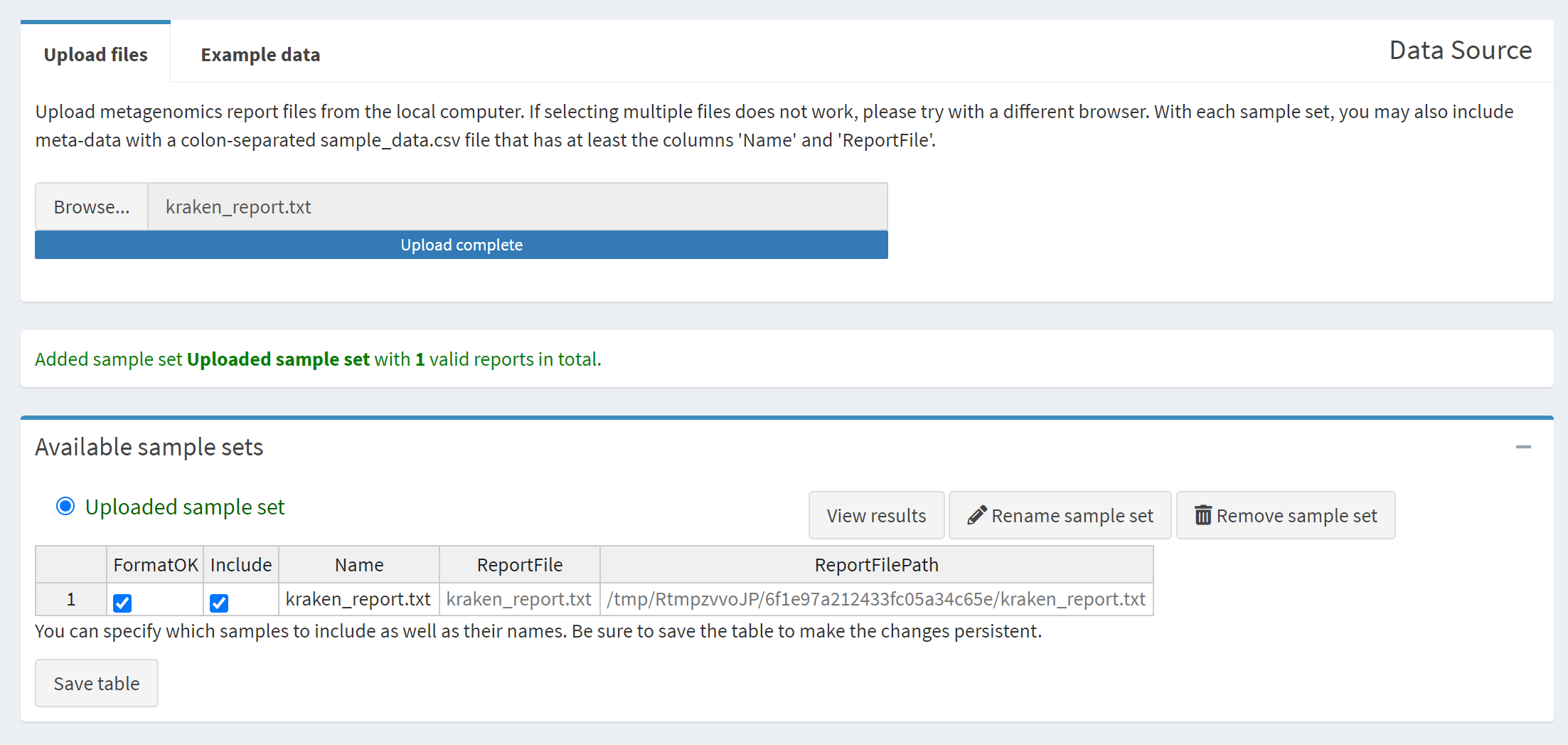
-
Select Generate HTML report … to generate the Pavian report.
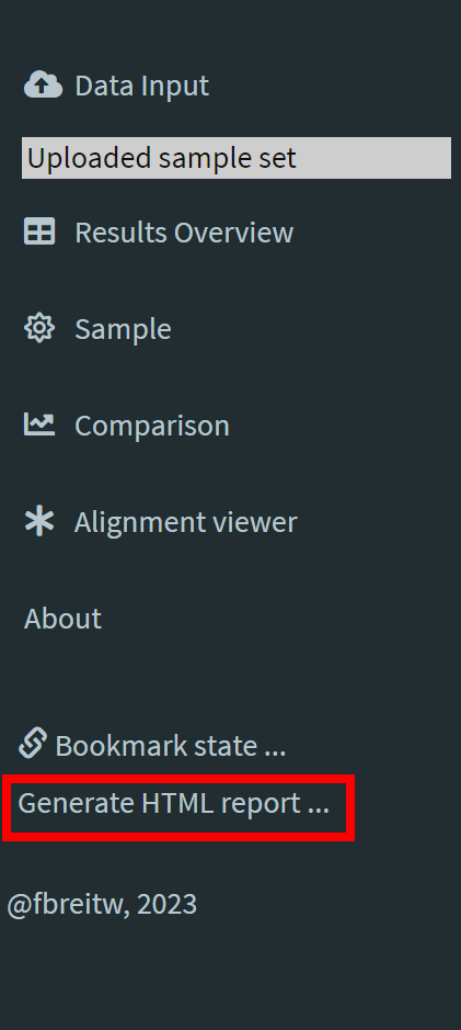
- Open the generated report HTML file in your web browser.
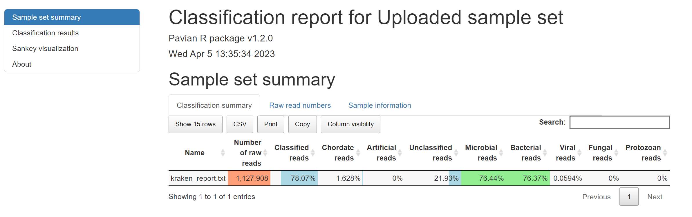
If all the steps are completed successfully then the report you should see should look like the following:
If something did not work, you can alternatively view a pre-computed report at http://xx.uhn-hpc.ca/module8_workspace/precomputed-analysis/Uploaded_sample_set-report.html.
Step 5: Questions
- What are the percentages of Unclassified, Microbial, Bacterial, Viral, Fungal, and Protozoan reads in this dataset?
- Scroll down to the Classification results section of the report and flip through the Bacteria, Viruses, and Eukaryotes tabs. What is the top organism in each of these three categories and how many reads?
- This data was derived from RNA (instead of DNA) and some viruses are RNA-based. If we focus in on the Viruses category, is there anything here that could be consistent with the patient’s symptoms?
- Given the results of Pavian, can you form a hypothesis as to the cause of the patient’s symptoms?
Assembly-based approach
Step 6: Metatranscriptomic assembly
In order to investigate the data further we will assemble the metatranscriptome using the software MEGAHIT. What this will do is integrate all the read data together to attempt to produce the longest set of contiguous sequences possible (contigs). To do this please run the following:
Commands
# Time: 6 minutes
megahit -t 4 -1 filtered.in.R1.fastq -2 filtered.in.R2.fastq -o megahit_out
If everything is working you should expect to see the following as output:
Output
2021-09-30 11:53:35 - MEGAHIT v1.2.9
2021-09-30 11:53:35 - Using megahit_core with POPCNT and BMI2 support
2021-09-30 11:53:35 - Convert reads to binary library
2021-09-30 11:53:36 - b'INFO  sequence/io/sequence_lib.cpp  :   75 - Lib 0 (/media/cbwdata/workspace/module8_workspace/analysis/filtered.in.R1.fastq,/media/cbwdata/workspace/module8_workspace/analysis/filtered.in.R2.fastq): pe, 2255816 reads, 151 max length'
2021-09-30 11:53:36 - b'INFO  utils/utils.h                 :  152 - Real: 1.9096\tuser: 1.8361\tsys: 0.3320\tmaxrss: 166624'
2021-09-30 11:53:36 - k-max reset to: 141
2021-09-30 11:53:36 - Start assembly. Number of CPU threads 4

[...]

2021-09-30 11:58:01 - Assemble contigs from SdBG for k = 141
2021-09-30 11:58:02 - Merging to output final contigs
2021-09-30 11:58:02 - 3112 contigs, total 1536607 bp, min 203 bp, max 29867 bp, avg 493 bp, N50 463 bp
2021-09-30 11:58:02 - ALL DONE. Time elapsed: 267.449160 seconds
Once everything is completed, you will have a directory megahit_out/ with the output. Let’s take a look at this now:
Commands
ls megahit_out/
Output
checkpoints.txt done final.contigs.fa intermediate_contigs log options.json
It’s specifically the final.contigs.fa file that contains our metatranscriptome assembly. This will contain the largest contiguous sequences MEGAHIT was able to construct from the sequence reads. We can look at the contents with the command head (head prints the first 10 lines of a file):
Commands
head megahit_out/final.contigs.fa
Output
>k141_0 flag=1 multi=3.0000 len=312
ATACTGATCTTAGAAAGCTTAGATTTCATCTTTTCAATTGGTGTATCGAATTTAGATACAAATTTAGCTAAGGATTTAGACATTTCAGCTTTATCTACAGTAGAGTATACTTTAATATCTTGAAGTACACCAGTTACTTTAGACTTAATCAAAATTTTACCCAAATCATTAACTAGATCTTTAGAATCAGAATTCTTTTCTACCATTTTAGCGATGATATCTGTTGCATCTTGATCTTCAAATGAAGATCTATATGACATGATAGTTTGACCTTCTTGTAGTTGAGATCCAACTTCTAAACATTCGATGTCT
>k141_1570 flag=1 multi=2.0000 len=328
GAGCATCGCGCAGAAGTATCTGTACTCCCTTTACTCCACGCAAGTCTTTCTCATACTCACGCTCGACACCCATCTTACCGATATAATCTCCCGGCTGATAGTACTCGTCTTCCTCAATATCACCCTGACTCACCTCTGCAACATCCCCAAGGACATGTGCAGCGATAGCTCGTTGATACTGACGAACACTACGTTTCTGAATATAAAAGCCTGGAAAACGATAGAGTTTCTCTTGGAAGGCGCTAAAGTCTTTATCACTCAATTGGCTCAAGAATAGTTGCTGCGTAAAGCGAGAGTAACCCGGATTCTTACTCCTATCCTTGATCCC
[...]
It can be a bit difficult to get an overall idea of what is in this file, so in the next step we will use the software Quast to summarize the assembly information.
Step 7: Evaluate assembly with Quast
Quast can be used to provide summary statistics on the output of assembly software. Quast will take as input an assembled genome or metagenome (a FASTA file of different sequences) and will produce HTML and PDF reports. We will run Quast on our data by running the following command:
Commands
# Time: 2 seconds
quast -t 4 megahit_out/final.contigs.fa
You should expect to see the following as output:
Output
/usr/local/conda/envs/module8-emerging-pathogen/bin/quast -t 4 megahit_out/final.contigs.fa

Version: 5.2.0

System information:
  OS: Linux-5.19.0-1022-aws-x86_64-with-glibc2.35 (linux_64)
  Python version: 3.9.16
  CPUs number: 4

Started: 2023-04-05 11:56:09

[...]

Finished: 2023-04-05 11:56:12
Elapsed time: 0:00:02.443741
NOTICEs: 1; WARNINGs: 0; non-fatal ERRORs: 0

Thank you for using QUAST!
Quast writes it’s output to a directory quast_results/, which includes HTML and PDF reports. We can view this using a web browser by navigating to http://xx.uhn-hpc.ca/module8_workspace/analysis/ and clicking on quast_results then latest then icarus.html. From here, click on Contig size viewer. You should see the following:
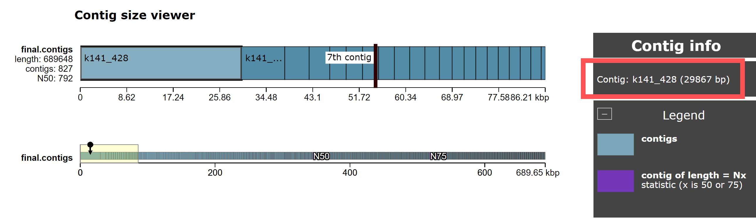
This shows the length of each contig in the megahit_out/final.contigs.fa file, sorted by size.
Step 7: Questions
- What is the length of the largest contig in the genome? How does it compare to the length of the 2nd and 3rd largest contigs?
- Given that this is RNASeq data (i.e., sequences derived from RNA), what is the most common type of RNA you should expect to find? What are the approximate lengths of these RNA fragments? Is the largest contig an outlier (i.e., is it much longer than you would expect)?
- Is there another type of source for this RNA fragment that could explain it’s length? Possibly a Virus?
- Also try looking at the QUAST report (http://xx.uhn-hpc.ca/module8_workspace/analysis/quast_results/latest/ then clicking on report.html). How many contigs >= 1000 bp are there compared to the number < 1000 bp?
Step 8: Use BLAST to look for existing organisms
In order to get a better handle on what the identity of the largest contigs could be, let’s use BLAST to compare to a database of existing viruses. Please run the following:
Commands
# Time: 1 second
seqkit sort --by-length --reverse megahit_out/final.contigs.fa | seqkit head -n 50 > contigs-50.fa
blastn -db ~/CourseData/IDE_data/module8/db/blast_db/ref_viruses_rep_genomes_modified -query contigs-50.fa -html -out blast_results.html
As output you should see something like (blastn won’t print any output):
Output
[INFO] read sequences ...
[INFO] 3112 sequences loaded
[INFO] sorting ...
[INFO] output ...
Here, we first use seqkit to sort all contigs by length with the largest ones first (seqkit sort --by-length --reverse ...) and we then extract only the top 50 longest contigs (seqkit head -n 50) and write these to a file contigs-50.fa (> contigs-50.fa).
Note that the pipe | character will take the output of one command (seqkit sort --by-length ..., which sorts sequences in the file by length) and forward it into the input of another command (seqkit head -n 50, which takes only the first 50 sequences from the file). The greater-than symbol > takes the output of one command seqkit head ... and writes it to a file (named contigs-50.fa).
The next command will run BLAST on these top 50 longest contigs using a pre-computed database of viral genomes (blastn -db ~/CourseData/IDE_data/module8/db/blast_db/ref_viruses_rep_genomes_modified -query contigs-50.fa ...). The -html -out blast_results.html tells BLAST to write its results as an HTML file.
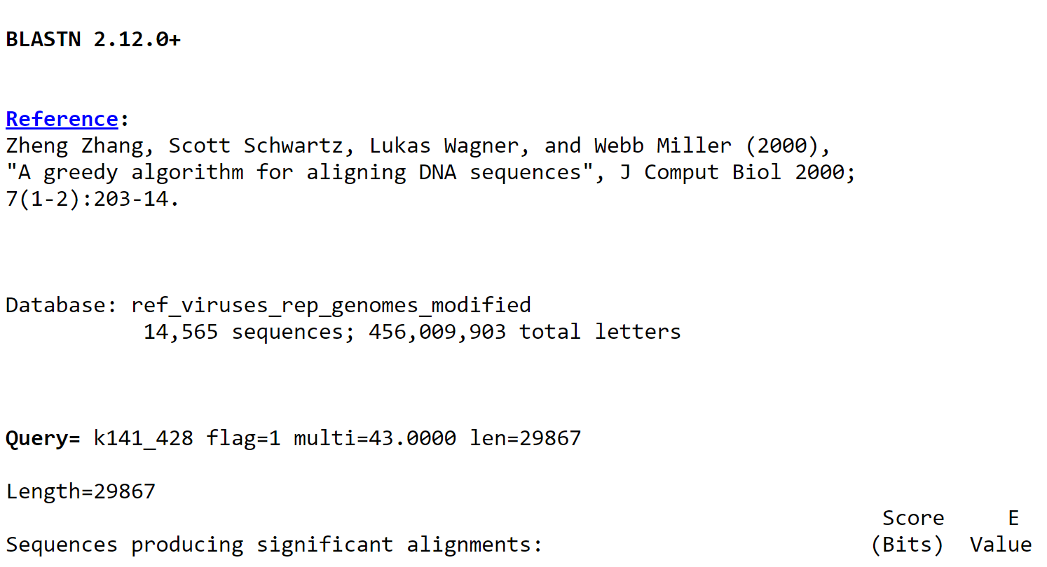
To view these results, please browse to http://xx.uhn-hpc.ca/module8_workspace/analysis/blast_results.html to view the ouptut blast_results.html file. This should look something like below:
Step 8: Questions
- What is the closest match for the longest contig you find in your data? What is the percent identify for this match (the value Z in
Identities = X/Y (Z%)). Recall that if a pathogen is an emerging/novel pathogen then you may not get a perfect match to any existing organisms. - Using the BLAST report alongside all other information we’ve gathered, what can you say about what pathogen may be causing the patient’s symptoms?
-
It can be difficult to examine all the contigs/BLAST matches at once with the standard BLAST report (which shows the full alignment). We can modify the BLAST command to output a tab-separated file, with one BLAST HSP (a high-scoring segment pair) per line. To do this please run the following:
Commands
blastn -db ~/CourseData/IDE_data/module8/db/blast_db/ref_viruses_rep_genomes_modified -query contigs-50.fa -outfmt '7 qseqid length slen pident sseqid stitle' -out blast_report.tsvThis should construct a tabular BLAST report with the columns labeled like
query id, alignment length, subject length, % identity, subject id, subject title. Taking a look at the fileblast_report.tsv, what are all the different BLAST matches you can find (the different values forsubject title)? How do they compare in terms of% identityandalignment length(in general, higher values for both of these should be better matches)?
5. Final words
Congratulations, you’ve finished this lab. As a final check on your results, you can use NCBI’s online tool to perform a BLAST on our top 50 contigs to see what matches to the contigs.
The source of the data and patient background information can be found at https://doi.org/10.1038/s41586-020-2008-3 (clicking this link will reveal what the illness is). The only modification made to the original metatranscriptomic reads was to reduce them to 10% of the orginal file size.
While we used MEGAHIT to perform the assembly, there are a number of other more recent assemblers that may be useful. In particular, the SPAdes suite of tools (such as metaviralspades or rnaspades) may be useful to look into for this sort of data analysis.
If you wish to see how the data (and databases) were generated for this example, please refer to the CourseData/IDE_data/module8/data-generation.md file.
As a final note, NCBI also performs taxonomic analysis using their own software and you can actually view these using Krona directly from NCBI. Please click here and go to the Analysis tab for NCBI’s taxonomic analysis of this sequence data (clicking this link will reveal what the illness is).