Module 5 Phylodynamics
Lab
Author: Angela McLaughlin and Finlay Maguire
Table of contents
1. Introduction
1.1. Background
SARS-CoV-2 Pango lineage B.1.1.7 (Rambaut et al. 2020) was the first officially designated variant of concern (VOC) by the World Health Organization (Konings et al. 2021), due to its increased transmissibility compared to other circulating lineages. Although B.1.1.7 was discovered in December 2020, it originated in the months preceding that. For a more thorough investigation into the circumstances of B.1.1.7 discovery and emergence, see (Hill et al., 2022) on “The origins and molecular evolution of SARS-CoV-2 lineage B.1.1.7 in the UK”.
Evaluating when and where (and in what host, for multi-host pathogens) novel lineages or variants with increased transmissibility or virulence emerge is important towards improving our understanding of the conditions supporting the emergence of variants against which pharmaceutical (vaccines, therapies) or non-pharmaceutical interventions may be less effective.
In this tutorial, we will analyze early SARS-CoV-2 B.1.1.7 sequences and associated metadata from the first months following its detection to reconstruct its likely time and place of origin using phylodynamics and phylogeography, in both maximum likelihood and Bayesian statistical frameworks.
1.2. Objectives of this analysis:
Download and clean publicly available SARS-CoV-2 B.1.1.7 sequences
Remove sequences with incomplete sample dates and subsample fewer sequences (keeping earliest with higher probability)
Align sequences and filter out low-quality sequences
Summarize the spatiotemporal distribution of samples
Infer a maximum likelihood phylogenetic tree (divergence tree)
Infer a maximum likelihood time-scaled tree using a molecular clock model
Conduct ancestral state reconstruction to identify the most likely geographic origin of lineage B.1.1.7
Compare the maximum likelihood estimates to those obtained in a Bayesian framework using Delphy
1.3. What statistical approach is best?
Maximum likelihood and Bayesian approaches to phylodynamics and phylogeography differ in their assumptions, algorithms, computational speed, scalability, and interpretation.
For large scale analyses (>10,000 sequences), maximum likelihood pipelines implemented in augur, treetime, iqtree, and R package ape, are more feasible, while analyses of smaller datasets (up to ~1000 sequences) can be done using Bayesian frameworks implemented in Delphy and BEAST, with the added benefits of incorporating uncertainty in the tree inference in parameter estimation and of specifying priors to limit the search space.
If you are interested in exploring more complex applications and methods for phylodynamic analyses, I recommend checking out resources from the “Taming the BEAST” workshops that are held semi-regularly, as well as he tutorials shared by the BEAST Developers. Paul Lewis’ phyloseminar.org lectures on Bayesian phylogenetics (part 1 and part 2) are also an excellent place to start to learn the basic theory of Bayesian methods.
Let’s go.
2. List of software for tutorial
3. Exercise setup
3.0. Data source
We will not spend time downloading the data, but rather will copy the datafiles as described in the subsequent section. However, it’s important to understand how this was done for the sake of reproducibility and interpretation.
Filters applied to download this dataset
SARS-CoV-2 B.1.1.7 (Alpha variant) data from NCBI Virus
- Pango lineage: B.1.1.7
- Host: human
- Dates:
- Collection date: Sep 1 2020 to Jan 1 2021 (First few months of detection)
- Release date: Sep 1 2020 to Jan 1 2022 (allow one year delayed submission)
- Sequence Quality:
- Nucleotide completeness: complete only
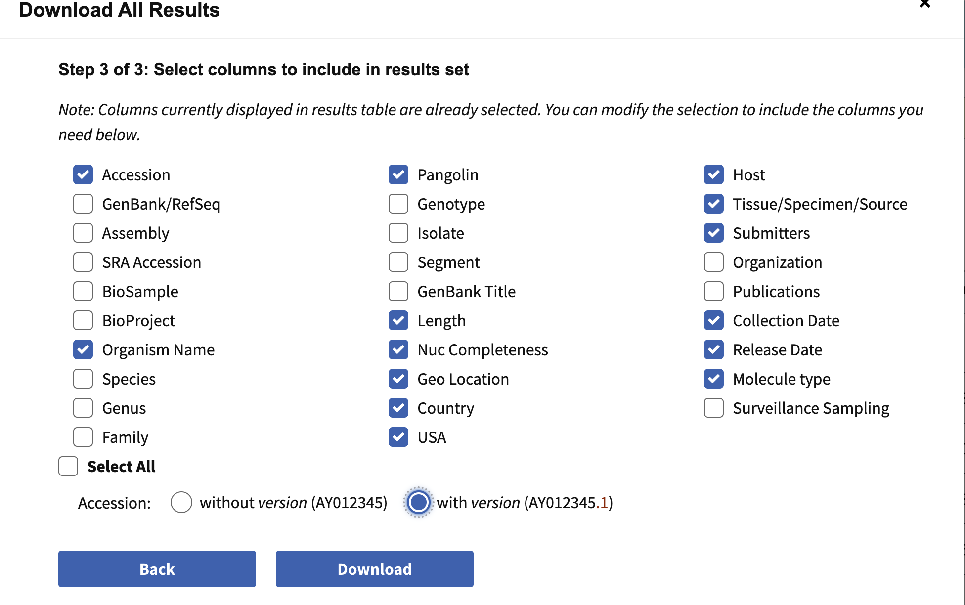
- Nucleotide > Download all results
- Data type
- sequence data = nucleotide; Fasta definition line: accession, country, collection date
- Results table in csv format; Results csv > Accession with version number
- N=15790 fasta sequences (b117_seq.fasta) and metadata (b117_seq.csv)
Information to include when downloading metadata from NCBI:
3.1. Copy data files
To begin, we will copy over the downloaded files to ~/workspace.
Commands
When you are finished with these steps you should be inside the directory /home/ubuntu/workspace/module5. You can verify this by running the command pwd.
Output after running pwd
/home/ubuntu/workspace/module5You should also see a directory data/ in the current directory which contains all the input data. You can verify this by running ls data/download:
Output after running ls data/download
b117_seq.csv b117_seq.fasta reference_MN908947.3.fasta It is also good to verify the data was copied fully. Run this code to count how many sequences are in the fasta file (each one starts with >): Commands
This should be 15790.
3.2. Activate conda environment
Next we will activate the conda environment, which will have all the tools needed by this tutorial pre-installed.
Commands
You should see the command-prompt (where you type commands) switch to include (sc2b117_phylodyn) at the beginning, showing you are inside this environment. You should also be able to run the augur command like augur --version and see output:
Output after running augur --version
augur 32.0.0 3.3. Find your IP address to setup an AWS instance
Similar to yesterday, we will want to either use the assigned hostname (e.g., xx.uhn-hpc.ca where xx is your instance number) or find the IP address of your machine on AWS so we can access some files from your machine on the web browser. To find your IP address you can run:
Commands
This should print a number like XX.XX.XX.XX. Once you have your address, try going to http://xx.uhn-hpc.ca and clicking the link for module5. This page will be referred to later to view some of our output files. In addition, the link precomputed-analysis will contain all the files we will generate during this lab (phylogenetic trees, etc).
3.4. Inspect and clean data
The first step of any phylogenetic analysis is to inspect and clean the dataset. Initial cleaning (before even looking at the sequence quality) steps include checking that accessions and sequence names are complete and unique, checking the completeness of sampling dates and locations (especially in phylodynamic analyses where these play a central role), checking the range of dates are realistic, and looking at how many geographic categories there are and whether some are more well-represented than others.
Run the following Rscript in the command line to de-duplicate seqeunces, remove incomplete dates, and subsample the data.
Commands
While this is running, let’s have a look inside the R script. Open the .Rproj file in RStudio, then open scripts/dedup_comp_dates.R. Note that while we have called this script from the command line, you can also run it within Rstudio by manually specifying the arguments.
What is happening inside this script:
- De-duplicate identical sequences (taking earliest collection date of replicates)
- Rename sequences without any spaces and add sequence name to metadata
- Identify and remove incomplete collection date (yyyy or yyyy-mm)
- Create a smaller subsampled dataset ‘complete_sampUK’ with equal number of non-UK and UK samples
- NOTE: this is the dataset that we will be working with in this lab due to limited time. In a more robust analysis, we would include more samples, repeat sampling with different seeds, and rather than sampling at random, we might consider sampling proportionally to geographies’ diagnosed cases through time to more accurately reflect spatiotemporal dynamics
- Export fasta and csv files into data/complete subfolder
Questions
- How many sequences were downloaded?
- How many sequences were there after de-duplicating?
- After de-duplicating, how many had complete dates? How many were sampled (sampUK)?
- How might you modify the subsampling scheme to reduce bias? to quantify uncertainty in the sampling process?
Answers
- n=15790
- n=14774
- n=10813; n=178
- Proportional to case counts through time and space. Multiple subsamples of different sizes or proportional contributions of countries.
Once that code is done, let’s run some R scripts from the command line to quickly summarize the number and/or proportion of sequences by country through time. Alternatively, in RStudio, go to file>new file>Rscript, copy/paste code chunk, save and run it there.
Commands
#
R

library(tidyverse)
library(RColorBrewer)

#data in
dat.samp<-read.delim("data/complete/b117_seq_complete_sampUK.tsv")
nrow(dat.samp)
dat.samp$date<-as.Date(dat.samp$date)

#range of dates
range(dat.samp$date)

#countries
t.c<-table(dat.samp$Country) %>% sort(decreasing = T);t.c
order.c<-names(t.c) #order of countries w/ most to least seqs/samples
n.c<-length(unique(dat.samp$Country));n.c

#more specific geos also available
table(dat.samp$Geo_Location) %>% sort(decreasing = T)
length(unique(dat.samp$Geo_Location))

#setup colors for countries
country.cols<-colorRampPalette(brewer.pal(n=8,name="Dark2"))(n.c)
names(country.cols)<-order.c

#factor and levels specifies order in legend
dat.samp$Country<-factor(dat.samp$Country, levels=order.c)

#plot country contribs
ggplot(dat.samp) +
  geom_bar(aes(x=Country, fill=Country))+
  theme_bw()+
  labs(x="Country", y="N sample", fill="Country")+
  scale_fill_manual(values=country.cols)+
  theme(axis.text.x=element_text(angle=45,vjust=1,hjust=1),
        legend.position="none")
ggsave(paste0("data/complete/samples_country.png"))

#plot it over time
ggplot(dat.samp) +
  geom_bar(aes(x=date, fill=Country))+
  theme_bw()+
  labs(x="Sample collection date", y="N sample", fill="Country")+
  scale_fill_manual(values=country.cols)

#save it
ggsave(paste0("data/complete/samples_time_country.png"))
If you are in command line R, enter q() to get out.
Questions
- How many sequences were included from the UK?
- What is the range of sample collection dates in the final dataset?
- How many countries were represented in the final dataset?
Answers
- 89
- 2020-09-20 to 2021-01-01
- 17 countries
4. Maximum likelihood phylodynamic analysis
The overall goal of this lab is to estimate where and when B.1.1.7 most likely originated. To do this, we will mostly make use of the Augur maximum likelihood tool suite, which powers the NextStrain website. Within augur, the key tool actually being used for most of our inferences is TreeTime a likelihood based tool for inferring molecular clocks and ancestral traits.
An overview of the basic usage of Augur (figure from the Augur documentation):
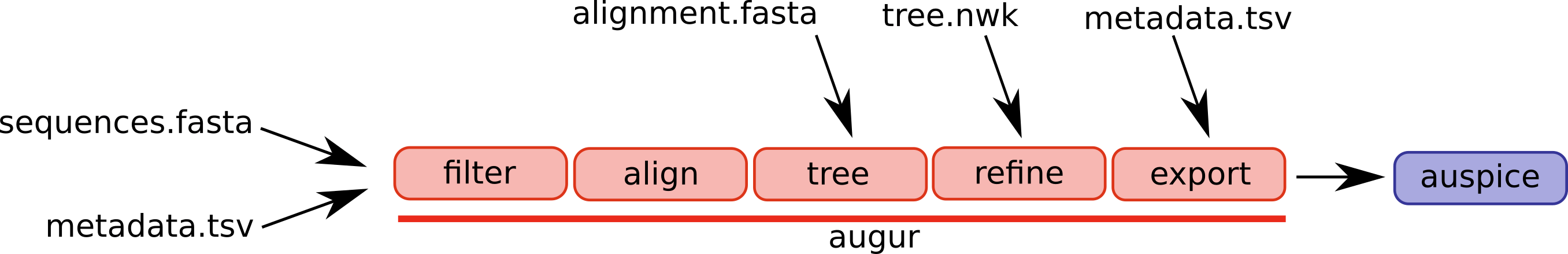
The steps/functions we use are in this section of the lab are the following:
- align: This step constructs a multiple sequence alignment from this subset of genomes.
- index: This step indexes the sequences, counting the frequency of nucleotides and gaps.
- filter: This step filters out sequences that have too many gaps or ambiguous nucleotides.
- tree: This step builds a phylogenetic tree, where branch lengths are measured in substitutions/site (a divergence tree).
- refine: This step constructs a time tree using our existing tree alongside collection dates of SARS-CoV-2 genomic samples (branch lengths are measured in time).
- traits: This step uses treetime’s mugration model to infer ancestral traits based on the tree. We will use this to infer ancestral host and geography.
- export: This step exports the data to be used by Auspice, a version of the visualization system used by NextStrain that lets you examine your own phylogenetic tree and metadata.
4.1. Construct a multiple sequence alignment of the genomes (augur align)
The first step is to construct a multiple sequence alignment of the genomes, which is required before building a phylogenetic tree. We will be using the command augur align to accomplish this task, but underneath this mafft runs to construct the alignment.
To build a new folder and construct the alignment, please run the following:
Commands
mkdir data/aligned

augur align --nthreads 2 --sequences data/complete/b117_seq_complete_sampUK.fasta --reference-sequence data/download/MN908947.3.fasta --output data/aligned/b117_seq_complete_sampUK_aligned.fasta
You should expect to see the following:
Output
using mafft to align via:
    mafft --reorder --anysymbol --nomemsave --adjustdirection --thread 2 data/b117_seq_complete_sampUK_aligned.fasta.to_align.fasta 1> data/b117_seq_complete_sampUK_aligned.fasta 2> data/b117_seq_complete_sampUK_aligned.fasta.log

    Katoh et al, Nucleic Acid Research, vol 30, issue 14
    https://doi.org/10.1093%2Fnar%2Fgkf436

WARNING: 1bp insertion at ref position 200 was due to 'N's or '?'s in provided sequences
WARNING: 1bp insertion at ref position 6337 was due to 'N's or '?'s in provided sequences
Trimmed gaps in MN908947.3|China|2019-12-26 from the alignment
The meaning of each parameter:
- `–nthreads: Number of threads for the alignment.
- `–sequences: The input set of sequences in FASTA format.
- `–output: The output alignment, in FASTA format.
- `–reference-sequence: The reference genome (MN908947.3==Wuhan-Hu-1).
The reference sequence will be included in our alignment and augur align removes any insertions with respect to this reference genome (useful when identifying and naming specific mutations later on in the augur pipeline).
The aligned fasta file is a very similar format as the input file, but the difference is that sequences have been aligned (possibly by inserting gaps -). This also means that all sequences in alignment.fasta should have the same length (whereas sequences in sequences.fasta, which is not aligned, may have different lengths). When time allows, it is good practice to visually inspect the alignment in a viewer such as AliView.
4.2. Index sequences (augur index)
This step is optional but useful to inspect sequence quality and quicken the subsequent filtering step, by counting the frequency of nucleotides and gaps.
Commands
augur index --sequences data/aligned/b117_seq_complete_sampUK_aligned.fasta --output data/aligned/b117_seq_complete_sampUK_aligned_sequence_index.tsvInspect the index output in the ‘aligned’ subfolder.
Questions
- Knowing that the genome size is 29,903 bp, do any samples appear to have more gaps or Ns than you would expect?
Answers
- At first glance, none appear to have >~3000 gaps or Ns.
4.3. Filter out low quality sequences (augur filter)
Filter seqs to a minimum length (–min-length) of 26913, which represents 90% of 29,903 sites with ACTG (i.e., max 10% ambig and gaps)
Commands
mkdir data/filtered

augur filter --nthreads 2 --sequences data/aligned/b117_seq_complete_sampUK_aligned.fasta --metadata data/complete/b117_seq_complete_sampUK.tsv --sequence-index data/aligned/b117_seq_complete_sampUK_aligned_sequence_index.tsv --min-length 26913 --output-sequences data/filtered/b117_seq_complete_sampUK_aligned_filt.fasta --output-metadata data/filtered/b117_seq_complete_sampUK_filt.tsv
Output
1 strain was dropped during filtering
    1 had no metadata (this is the refence sequence)
178 strains passed all filters
Nice, all the sequences passed our quality filters (this is rarer than you might think).
Questions
- Why is it important to remove low quality sequences prior to phylogenetic inference?
- The choice of maximum 10% ambiguous and gaps seems (is) somewhat arbitrary. How would increasing or decreasing this threshold change the analysis?
Answers
- Sequences with excessive gaps or ambiguous sites may not have as high of accuracy, and have less signal to contribute to the tree, which could bias its placement.
- Increasing the threshold would allow more sequences of lower quality to pass through the filter. Decreasing the threshold is more conservative.
4.4. Mask problematic sites in the alignment
Not all sites in the genome are equally informative towards inferring their phylogenetic relationships. Some sites can be misleading and should be masked before building trees. The ends of alignments often exhibit low coverage and a higher rate of sequencing or mapping errors. In SARS-CoV-2, this includes positions 1–55 and 29804–29903. Homoplasic sites at which multiple recurrent mutations arise may reflect contamination, recurrent sequencing errors, or hypermutability. Even if they are accurate, they may not be representative of evolution across the remainder of the genome. Another example (not relevant here) would be sites at which drug resistance mutations occur. In HIV-1 phylodynamic analyses, codons of surveillance drug resistance mutations are masked. For further interest, see this justification for masking SARS-CoV-2 sequences.
Note that augur also has a masking subcommand, but it requires the mask file to be in a different format, so we’re not using it here. Instead, we’re going to run a python script that masks sequences based on a vcf (Variant Call Format) file of problematic sites. In order to run this, we have to concatenate the reference sequence back into the fasta, which was filtered out by augur above. Then we’re going to run our masking script, and then remove that reference again.
Commands
mkdir data/masked

## Concatenate the fasta with the reference fasta
cat data/filtered/b117_seq_complete_sampUK_aligned_filt.fasta data/download/MN908947.3.fasta > data/filtered/b117_seq_complete_sampUK_aligned_filt_ref.fasta

## Run the masking python script
python3 scripts/mask_alignment_using_vcf.py -i data/filtered/b117_seq_complete_sampUK_aligned_filt_ref.fasta -o data/masked/b117_seq_complete_sampUK_aligned_filt_ref_mask.fasta -v scripts/problematic_sites_vcfv5.vcf -n "n" --reference_id "MN908947.3|China|2019-12-26"

## Remove the reference sequence from the alignment using augur filter
augur filter --sequences data/masked/b117_seq_complete_sampUK_aligned_filt_ref_mask.fasta --metadata data/filtered/b117_seq_complete_sampUK_filt.tsv --output-sequences data/masked/b117_seq_complete_sampUK_aligned_filt_mask.fasta --output-metadata data/masked/b117_seq_complete_sampUK_aligned_filt_mask.tsv
The $cat command is a simple and useful tool to concatenate multiple fasta files together.
Let’s have a closer look at the parameters we used in the python script:
-i: Fasta input alignment to be masked (with the ref sequence in it)-o: Fasta output alignment with problematic sites masked-v: The vcf file of problematic sites from de Maio-n: the character to replace nucleotides at the masked sites--reference-id: the ID of the reference sequence in the input
4.5. Build a maximum liklihood phylogenetic tree (augur tree)
The next step is to take the set of aligned genomes and build a phylogenetic tree (a divergence tree in units of substitutions per site). We will use augur tree for this, but underneath it (by default) runs iqtree, which uses maximum likelihood to infer a phylogenetic tree.
Commands
mkdir trees

augur tree --nthreads 4 --method iqtree --substitution-model GTR --alignment data/masked/b117_seq_complete_sampUK_aligned_filt_mask.fasta --output trees/b117_seq_complete_sampUK_aligned_filt_mask.tre
Let’s check out the parameters
--nthreads: Number of threads--method: The tree inference method. We use the default, iqtree(3)--substitution-model: the underlying substitution model, here specified as generalized time reversible (GTR), which means that each nucleotide substitution rate in the matrix (ACTG vs ACTG) is separately estimated.--alignment: the input alignment (with masked sites)--output: the output tree (can be .tre or .nwk files)
You should expect to see this (or a very similar) output:
Output
Building a tree via:
    iqtree3 --threads-max 4 -s data/masked/b117_seq_complete_sampUK_aligned_filt_mask-delim.fasta -m GTR --ninit 2 -n 2 --epsilon 0.05 -T AUTO --redo > data/masked/b117_seq_complete_sampUK_aligned_filt_mask-delim.iqtree.log
    Please use the corresponding citations according to
    https://iqtree.github.io/doc/Home#how-to-cite-iq-tree

Building original tree took 12.720907926559448 seconds
This produces as output a .tre file, which is a Newick format phylogenetic tree, which has been midpoint-rooted. You can load this file in a variety of phylogenetic tree viewers (such as http://phylo.io/) but we will further refine this file to work with Auspice.
Another output file is alignment-delim.iqtree.log, which contains additional information from iqtree. You can take a look at this file to get an idea of what iqtree was doing by using tail (prints the last few lines of a file).
Commands
Output
Optimal log-likelihood: -44067.898
Rate parameters:  A-C: 0.24165  A-G: 1.07984  A-T: 0.21863  C-G: 0.31202  C-T: 3.23196  G-T: 1.00000
Base frequencies:  A: 0.299  C: 0.184  G: 0.196  T: 0.321
Parameters optimization took 1 rounds (0.019 sec)
BEST SCORE FOUND : -44067.898
Total tree length: 0.012

Total number of iterations: 2
CPU time used for tree search: 1.277 sec (0h:0m:1s)
Wall-clock time used for tree search: 0.408 sec (0h:0m:0s)
Total CPU time used: 29.925 sec (0h:0m:29s)
Total wall-clock time used: 12.023 sec (0h:0m:12s)

Analysis results written to:
  IQ-TREE report:                data/masked/b117_seq_complete_sampUK_aligned_filt_mask-delim.fasta.iqtree
  Maximum-likelihood tree:       data/masked/b117_seq_complete_sampUK_aligned_filt_mask-delim.fasta.treefile
  Likelihood distances:          data/masked/b117_seq_complete_sampUK_aligned_filt_mask-delim.fasta.mldist
  Screen log file:               data/masked/b117_seq_complete_sampUK_aligned_filt_mask-delim.fasta.log

Date and Time: Wed Nov 19 15:50:14 2025
As iqtree uses a maximum likelihood approach, you will see that it will report the likelihood score of the optimal tree (reported as log-likelihoods since likelihood values are very small).
Note: For this lab we are not looking at branch support values for a tree, but for real-world analysis you may wish to look into including (ultra-fast) bootstrap support values or approximate likelihood ratio test values. This will give a measure of how well-supported each branch in the tree is by the alignment (often a number from 0 for little support to 100 for maximal support). Please see the IQTree documentation for more details.
4.6. Inferring timing of host change (augur refine)
The tree output by iqtree shows hypothetical evolutionary relationships between different SARS-CoV-2 genomes with branch lengths representing distances between different genomes (in units of substitutions/site, i.e., the predicted number of substitutions between genomes divided by the alignment length). However, other methods of measuring distance between genomes are possible. In particular we can incorporate the collection dates of the different SARS-CoV-2 genomes to infer a tree where branches are scaled according to the elapsed time and the dates of internal nodes are inferred. Such trees are called time trees or time-scaled phylogenies.
We will use TreeTime invoked by augur to infer a time tree from our phylogenetic tree using collection dates of the SARS-CoV-2 genomes stored in the metadata file. We will use the augur refine step to run TreeTime and perform some additional refinemint of the tree.
To do this, please run the following:
Commands
augur refine --alignment data/masked/b117_seq_complete_sampUK_aligned_filt_mask.fasta --tree trees/b117_seq_complete_sampUK_aligned_filt_mask.tre --metadata data/masked/b117_seq_complete_sampUK_aligned_filt_mask.tsv --timetree --divergence-units mutations --output-tree trees/b117_seq_complete_sampUK_aligned_filt_mask_timetree.tre --output-node-data trees/refine.node.json --seed 123 --stochastic-resolve --root least-squares --date-confidence --clock-rate 4.5e-4 --clock-std-dev 0.2Once again, let’s have a closer look at the parameters:
--alignment: The alignment used to build the tree. Used to re-scale the divergence units.--tree: The starting input tree built using iqtree3.--metadata: The metadata which contains the SARS-CoV-2 genome names (in a column calledname) and the sample collection dates (in a column nameddate).--timetree: Specifiy to build a time tree.--divergence-units: Convert the branch lengths of substitutions/site (mutations/site) to mutations (not needed to build a time tree, this is just used for visualizing the tree later on).--output-tree: The output Newick file containing the time tree.--output-node-data: Augur will store additional information here which will let us convert between time trees and substitution trees.--seed: Set a seed for reproducibility--stochastic-resolve: Resolve polytomies stochastically (forces a bifurcating tree)--root: choose root that optimizes the least squares for the root-to-tip regression -date-confidence--clock-rate: We are specifying a relaxed molecular clock rate, with a mean of 4.5e-4 based on Hill et al. 2022--clock-std-dev: This is the deviance on the relaxed clock, allowing for variable evolutionary rates across the tree. You could play with this parameter if you have time.
You should expect to see the following as output:
Output
augur refine is using TreeTime version 0.11.4

4.28    TreeTime.reroot: with method or node: least-squares

4.28    TreeTime.reroot: rerooting will account for covariance and shared ancestry.

5.32    ###TreeTime.run: INITIAL ROUND

9.24    TreeTime.reroot: with method or node: least-squares

9.24    TreeTime.reroot: rerooting will account for covariance and shared ancestry.

9.41    ###TreeTime.run: rerunning timetree after rerooting

13.59   ###TreeTime.run: ITERATION 1 out of 2 iterations

21.88   ###TreeTime.run: ITERATION 2 out of 2 iterations

55.09   ###TreeTime.run: FINAL ROUND - confidence estimation via marginal
        reconstruction
Inferred a time resolved phylogeny using TreeTime:
    Sagulenko et al. TreeTime: Maximum-likelihood phylodynamic analysis
    Virus Evolution, vol 4, https://academic.oup.com/ve/article/4/1/vex042/4794731

updated tree written to trees/b117_seq_complete_sampUK_aligned_filt_mask_timetree.tre
node attributes written to refine.node.json
As output, the file output-tree trees/b117_seq_complete_sampUK_aligned_filt_mask_timetree.tre will contain the time tree while the file trees/refine.node.json contains additional information about the tree. If you want, download the time tree and view it in icytree.
4.7. Infer ancestral states for host and location (augur traits)
We will now be using treetime’s mugration model to reconstruct discrete ancestral states. In other words, we are trying to use the tree and genome metadata to reconstruct the most likely country at each of the internal nodes in the tree. It is called a mugration model because it is fundamentally estimating migration between “demes” (in this case, countries) as if it were a substitution rate matrix, commonly referred to as mu. See Lemey et al. 2009 if you’re interested in learning more.
Side bar: discrete phylogeography, ancestral state reconstruction, ancestral trait inference, and ancestral character estimation can all be used interchangeably in this context.
As with the other analyses, augur makes this process very convenient:
Commands
augur traits --tree trees/b117_seq_complete_sampUK_aligned_filt_mask_timetree.tre --metadata data/masked/b117_seq_complete_sampUK_aligned_filt_mask.tsv --columns Country Geo_Location --output-node-data trees/trait.node.jsonThe parameters we used are:
--tree: The time-calibrated tree we inferred in step 4--metadata: The metadata file with information about the genomes in the tree--columns: The columns in the metadata file we want to infer ancestral states for, in this case country and geo_location (more specific info).--output-node-data: Augur stores the additional information related to the ancestral trait inference for later visualisation.
You should expect to see the following as output:
Output
augur traits is using TreeTime version 0.11.4
Assigned discrete traits to 178 out of 178 taxa.

Assigned discrete traits to 178 out of 178 taxa.

Inferred ancestral states of discrete character using TreeTime:
    Sagulenko et al. TreeTime: Maximum-likelihood phylodynamic analysis
    Virus Evolution, vol 4, https://academic.oup.com/ve/article/4/1/vex042/4794731

results written to trait.node.json
4.8. Package up data for Auspice visualisation (augur export)
We will be using Auspice to visualize the tree alongside our metadata. To do this, we need to package up all of the data we have so far into a special file which can be used by Auspice. To do this, please run the following command:
Commands
augur export v2 --tree trees/b117_seq_complete_sampUK_aligned_filt_mask_timetree.tre --node-data trees/refine.node.json trees/trait.node.json --maintainers "CBW-IDE-2025" --title "Module 5 Practical" --output trees/analysis-package.json --geo-resolutions CountryThe parameters:
--tree: The time-calibrated tree--node-data refine.node.json trait.node.json: The 2 jsons created during the temporal and ancestral trait inference--title "Module 5 Practical": A title for the auspice page, you can make this anything you want.--maintainers "CBW-IDE-2025": A name for who is responsible for this analysis, useful for later, can make this anything you want.--geo-resolutions Country: Spatial resolution on which to plot the data. In this case we want country--output analysis-package.json: The key output file we want to generate. The filetrees/analysis-package.jsoncontains the tree with different branch length units (time and substitutions), our inferred ancestral traits, as well as additional data.
You should expect to see the following as output:
Output
Trait 'Geo_Location' was guessed as being type 'categorical'. Use a 'config' file if you'd like to set this yourself.
Trait 'Country' was guessed as being type 'categorical'. Use a 'config' file if you'd like to set this yourself.
Validating produced JSON
Validating schema of 'trees/analysis-package.json'...
Validating that the JSON is internally consistent...
Validation of 'trees/analysis-package.json' succeeded.
5. Visualizing the phylodynamic analysis
Now that we’ve constructed and packaged up a tree (analysis-package.json), we can visualize this data alongside the data augur has extracted from our metadata using augur and Auspice.
Note: I’ve had issues recently getting this to work in firefox so recommend using a chromium-based browser if you have issues.
5.1. Load data into Auspice
To do this, please navigate to http://IP-ADDRESS/module5/ and download the files trees/analysis-package.json and data/masked/b117_seq_complete_sampUK_aligned_filt_mask.tsv to your computer (if the link does not download you can Right-click and select Save link as…).
Next, navigate to https://auspice.us/ and drag the file analysis-package.json onto the page.
5.2. Explore data
Spend some time to explore the data and get used to the Auspice interface. Try switching between different Tree Layouts, Branch Lengths, or colouring the tree by different criteria in the metadata table. This is always worth doing a bit before diving into analyses. Scroll down and hit download to save the outputs of this for future reference. The nexus trees contain the internal node states along with the tree, so is readable into R and FigTree if you want to customize the tree more or analyze ancestral state transitions to identify sublineages or calculate dispersion rates etc.
5.3. Examine the molecular clock
Now we are going to look more at the Branch length “TIME” and “DIVERGENCE” option.
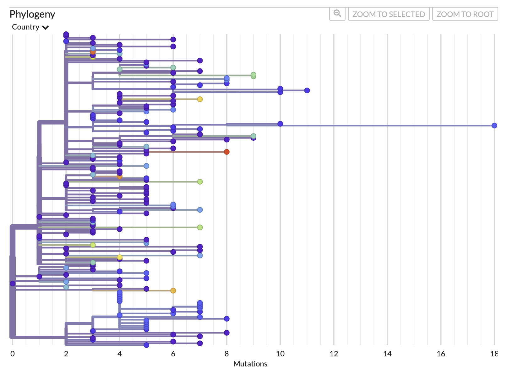
First, let’s look at the divergence tree and use the x-axis to work out how many mutations there are on certain branches. We can use the x-axis in the “RECTANGULAR” layout of the “DIVERGENCE” tree to work this out or we can directly move our cursor over the node/branch of interest to have a pop-up with the details.
The mutation tree:
Now, we can do the same thing if we switch to “TIME” and look at the approximate inferred dates of the internal nodes of the tree. We can also mouse over to get the exact pop-up dates.
Questions
- What was the maximum number of mutations from the root to any tip?
- What was the most likely date of the root (AKA the time of the most recent common ancestor (TMRCA)) ? Confidence interval?
- How do you interpret the root of this phylogeny? Is it representative of the entire B.1.1.7 lineage?
Answers
- 18 (to tip MW598424.1/Ghana/2020-12-22). This tip could be considered a temporal outlier and excluded from the analysis.
- 2020-08-21, but the confidence interval is wide and lower bound is unrealistic (2016-05-31 - 2020-09-12)
- This root is the most recent common ancestor (MRCA) of a random sample of early B.1.1.7 sequences, downsampling the UK samples to an equal number as non-UK samples. It may not be fully representative of the full diversity of early B.1.1.7, nor later evolution of B.1.1.7.
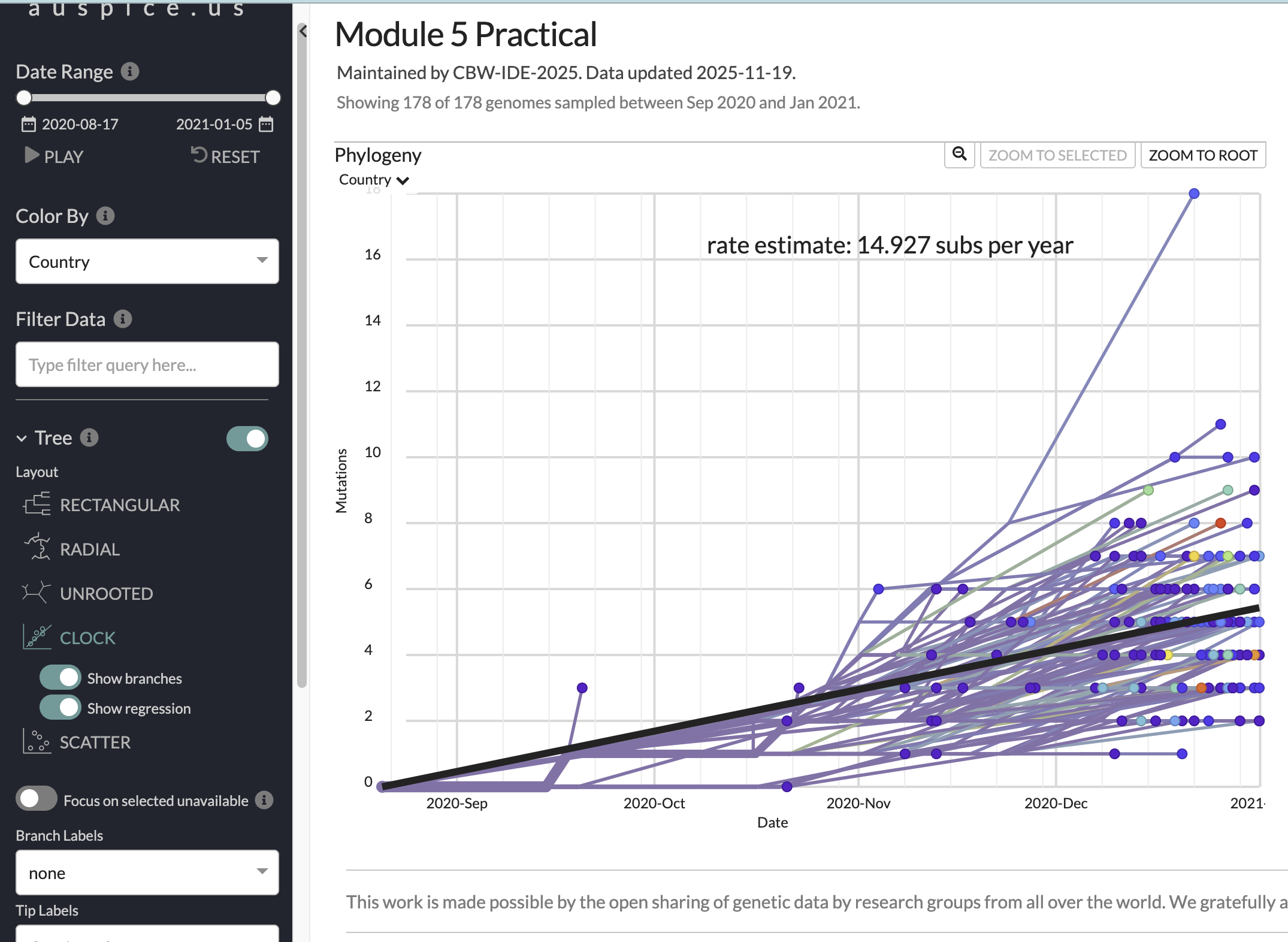
Now, have a look at the “CLOCK” layout/figure found in the options bar on the left of your screen. This brings up a root-to-tip regression from the divergence tree (i.e., how many mutations from root to tip, versus collection date). You can click on individual points (including the upper outlier from Ghana) to see the average substitution rate for that tip. for that tip.
The root-to-tip regression plot:
Questions
- What is the slope of the root-to-tip regression (in subs/year; subs/site/year)? What does it represent?
- Does the trend line for the root-to-tip regression look like a good fit with good temporal signal?
- Given the data and trendline, how accurate do you think the inferred root date is?
- How might you estimate the uncertainty in these estimates?
Answers
- 14.9 substitutions per year. Or (ignoring masked sites), 14.9/29903=0.0004982778=5.0 subs/site/year. It represents the strict molecular clock rate.
- Aside from the outlier, it looks like a good fit (an R-squared value should really be reported) with reasonable temporal signal.
- The confidence interval on the root is wide, we have a relatively small (singular) sample, but the linear fit is decent and we included early samples with higher probabilities, so I’d say medium to low accuracy for the mean estimate.
- Multiple subsamples of higher sample sizes. Bootstrapping/ultrafast bootstrapping. Multiple clock rate assumptions when inferring the time tree.
5.4. Examine the ancestral state reconstruction
We can colour the tree and rename the tree tip labels using the metadata to reflect the ancestral state reconstruction. The internal nodes/branches will be coloured based on the inferred ancestral state, in this case Country or Geo_location. Investigate the ancestral states at internal nodes throughout the tree including at the root. Use the play button to visualize the dispersion globally.
Here is a look at what you should be seeing in auspice when you change branches to be colored by Country and choose the multi-panel layout.
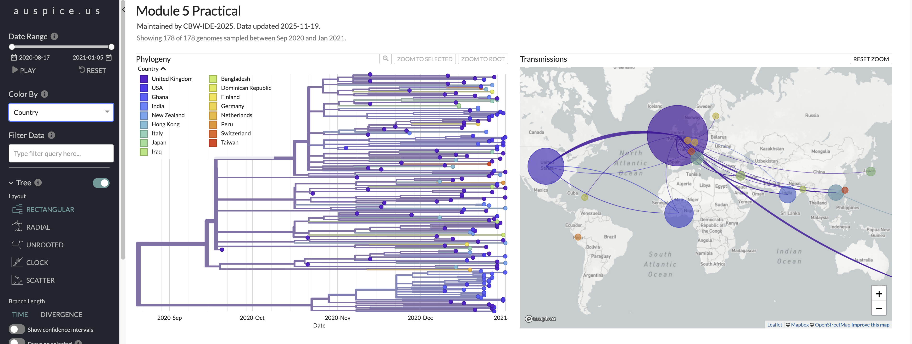
Questions
- Based on this analysis, where was the root of B.1.1.7 likely to have occurred?
- How do you think sequence subsampling might have impacted this analysis?
- What additional data would give you more confidence in asserting where this lineage was likely to have originated?
- How could you use the output of this analysis to quantify viral dispersion?
Answers
- The United Kingdom
- We included far fewer sequences from the UK than were available, and still inferred it as the likely origin. It would be worth comparing other sampling schemes to validate this, but we have high confidence that this was the likely origin, given the sequences publicly available.
- More early B.1.1.7 sequences from other countries would be informative. Also, including close parental or sister lineages (like B.1 similar to B.1.1.7) of similar time/place could add resolution to the analysis.
- Quantify importation or exportation rates by country through time. You could also incorporate population size, connectivity (mobility data), geographical distance, and other factors to evaluate (or control for) factors associated with elevated dispersal.
That’s that for our maximum likelihood phylogeographic inference. Now, we’re going to compare those results to a Bayesian approach.
6. Delphy analysis
Delphy is a newly released Bayesian phylogenetics tool designed to be fast, scalable, accessible, and accurate. Delphy is faster than other Bayesian tools because it uses Explicit Mutation-Annotated Trees (EMAT), which are hypotheses of how an ancestral sequence replicated and evolved, mutation by mutation, into the observed dated sequences. Check out their pre-print if you want more details.
In Bayesian phylogenetic (and phylodynamic) inference, many models (made up of trees and parameters) are sampled to generate posterior probability distributions, and our estimates will reflect the highest posterior density (HPD). Bayesian analyses differ from max likelihood approaches in that they incorporate uncertainty from the tree inference and sampling process, and rely on specification of prior probabilities for the parameters to be explored using Markov Chain Monte Carlo (MCMC), which is basically a hill-climbing algorithm that suggests and compares models compared to the previous step. Model convergence is assessed using minimum effective sampling size (ESS) reflects and in robust analyses is usually ~200 after removing the burn-in. Burn-in are steps that you don’t include in the final posterior distributions because they represent the model stabilization period. In a robust Bayesian analyses, multiple MCMC chains are run, and then combined after burn-in.
The tree displayed reflects a maximum clade credibility tree, which is a single tree with the highest posterior probability across the Bayesian posterior distribution of trees. Branch width represents the credibility threshold, more commonly referred to as posterior support or probability, which indicate the strength of evidence for clades, given the data and model used.
6.1. Modify fasta names, then load the renamed fasta into Delphy
Delphy wants sequence names to include info separated by “|” not “/”, so we’ll start by running a simple R script to rename the relevant fasta and metadata.
Run this Rscript in the command line. You can go to scripts/convert_names.R to have a look at what this script does, but it’s pretty simple.
Rscript scripts/convert_names.R "data/masked/b117_seq_complete_sampUK_aligned_filt_mask.tsv" "data/masked/b117_seq_complete_sampUK_aligned_filt_mask.fasta"The renamed files output goes to a newly created folder, data/delphy.
Now, open the Delphy web browser and drag/drop or upload the fasta file data/delphyb117_seq_complete_sampUK_aligned_filt_mask_delphy.fasta.
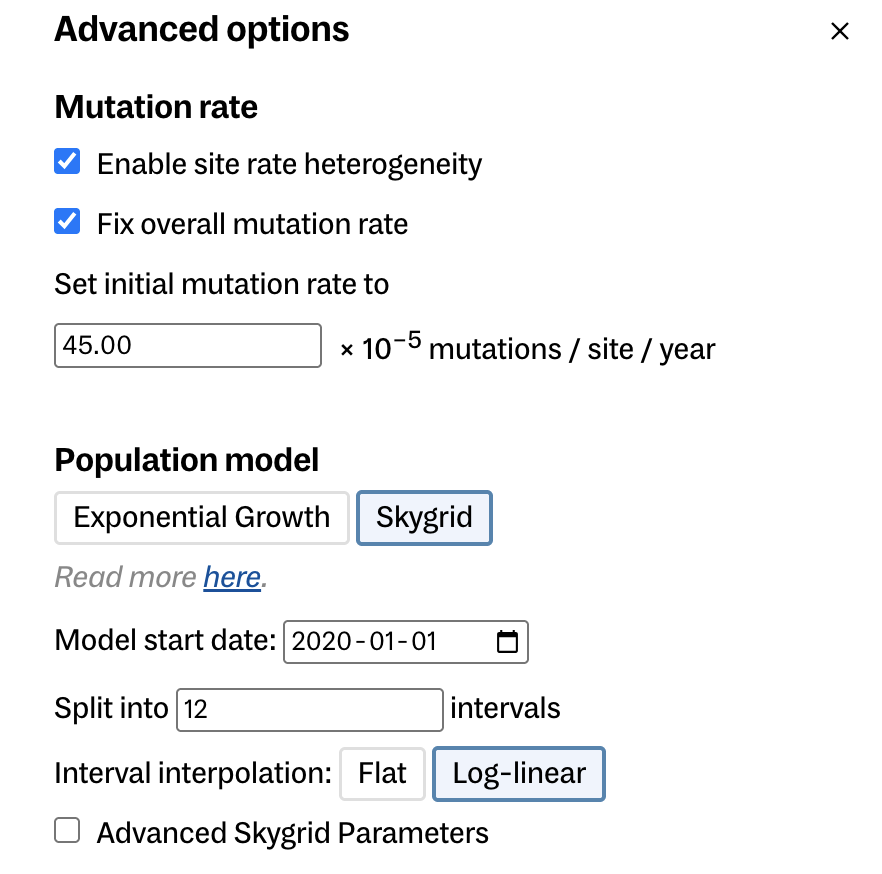
6.2. Modify priors by clicking on advanced options
Leave the sampling frequency to sample 1 tree per 1,000,000 steps. You could change this to sample more frequently if you want, but this might not improve the speed of convergence if trees are too similar to each other.
Let’s modify the priors. It is important to assess and modify priors in Bayesian analyses to reflect your prior expectations and narrow the parameter space explored. Improper priors not only slow down convergence, but can bias analyses.
- For mutation rate:
- enable site rate heterogeneity
- fix overall (mean) mutation rate
- set initial mutation rate to 45e-5 s/s/y 4.5e-4 (Hill et al. 2022)
- Population model
- Choose skygrid (these are both coalescent tree priors. Delphy does not have birth-death models like BEAST does.)
- model start date 2020-01-01 (the earliest this lineage root could have occurred)
- split into 10 intervals
- keep other parameters the same (could play with advanced skygrid parameters)
Here is a look at the advanced options you should be modifying. This should also have had split into 10 intervals.
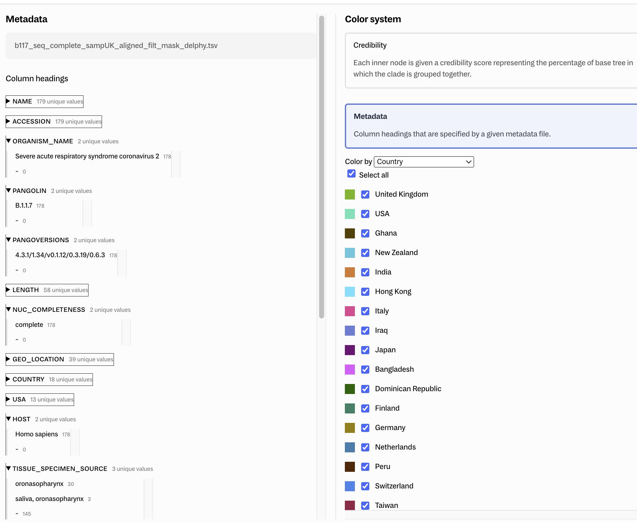
Before we start the run, go to Customize in the toolbar, then add the metadata file data/delphyb117_seq_complete_sampUK_aligned_filt_mask_delphy.tsv by drag/drop then in Color system, click metadata, color by Country, then select all.
Delphy customize options:
Questions
- what biases may we have imposed through our selection of priors?
Answers
- We may bias our estimates of the root date by specifying an improper mean molecular clock rate. The skygrid may not fit well with 10 categories (not enough data in early period). The underlying population may be better described by the exponential population distribution. Any misspecified or over-generalized prior has the potential to bias the analysis or underestimate the true uncertainty in the estimates.
6.3. Run the analysis and interpret output
Hit play and watch in statistical awe as trees sampled from the posterior are displayed in real-time, alongside model parameters including the number of mutations, ln(posterior), total evolutionary time (tree height), and effective population size in years. We can start to investigate the output before the run is complete (or you can upload the precomputed-analysis/trees/delphy_out/.delphy file directly to the Delphy home page to analyze a more complete analysis of >300 million steps).
Here is a look at the more complete run, including a sampled tree, the MCC tree, and the posterior distribution of some key model parameters.
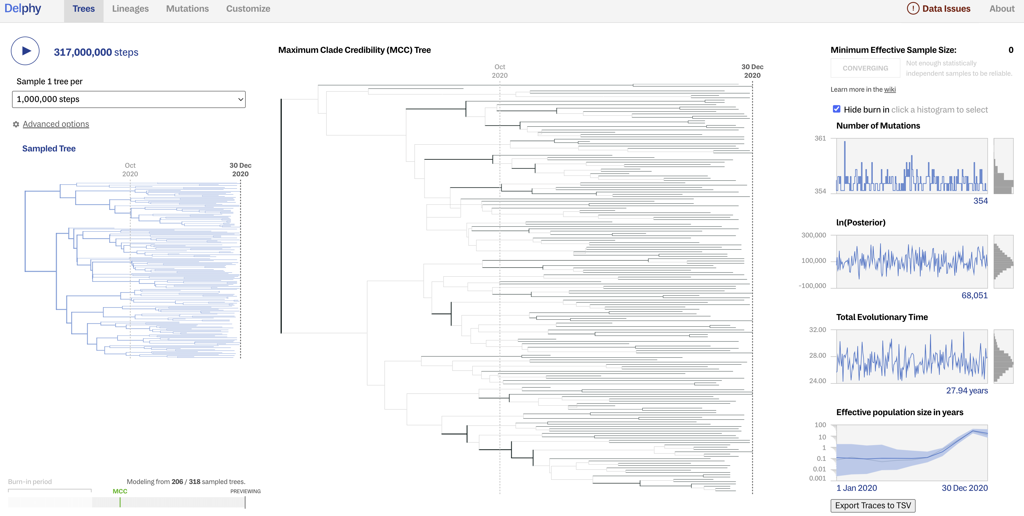
Although Delphy does not seem very good at estimating the ESS and assessing convergence, a good sign of convergence is when the posterior distributions of parameters appear as “fuzzy caterpillars” (converging around similar values, as opposed to jumping around).
Questions
How do you interpret the change in effective population size through time?
Did your model converge? How can you tell?
Answers
The effective population size is low and then increases rapidly (exponentially?) as this lineage transmitted broadly in the UK and globally, but then appears to decrease at the end of the study perio, but this likely reflects lower sampling rate towards the end of the period.
After removing burn-in, the ESS for the parameters shown are below 200, so probably not. We would have to run this for more steps, and maybe for multiple chains that we could combine using a tool like Tracer.
NEXT, let’s click on Lineages in the upper tool bar. In the bottom left corner, you can change branch coloring between Credibility and Metadata (Country). You can also change the credibility threshold (posterior support) for nodes’/branches’ shading in the tree displayed.
Questions
Is the first bifurcation at the root well-supported?
What is the median posterior root date?
Answers
No, the credibility threshold is <50%.
Median posterior root date ~19 July 2020. Normally a 95% HPD should be reported, but Delphy does not show that directly. If you have time/interest, you can read the exported data into R and estimate the uncertainty.
And now click on Mutations in the upper tool bar. Click on recurrent mutations, then A17615G. This mutation may have evolved independently multiple times, though it was only found in 70 genomes. It is a non-synonymous mutation in the ORF1b gene, resulting in an amino acid change of Lysine to Arginine (K1383R) in the nsp10 protein. Explore the other mutations that occurred in the phylogeny.
Questions
Where does the Delphy analysis suggest the root of this B.1.1.7 phylogeny occurred?
Does the Bayesian analysis corroborate the maximum likelihood analysis in terms of the time and place of origin of B.1.1.7?
Answers
The UK
Yes! Both the Bayesian and ML analyses suggest this lineage originated around August 20, 2020 in the UK. This is very close to the estimate from Hill et al. 2022 of a “TMRCA of the Alpha clade estimated at 28 August 2020 (95 % HPD: 15th August 2020 to 9th September 2020)”.
6.4. Export results
To wrap this Delphy analysis up, go to Customize, then in the bottom left, export the Tree as png and Newick file, and the Delphy run. The Delphy run file can be dropped back into Delphy or read into R. You can also generate input/output to BEAST to run a more bespoke Bayesian analysis.
7. End of lab
You’ve made it to the end of the lab. Awesome job.
You deserve a little treat

If you have some extra time, you can explore Auspice or Delphy further, or see how the results differ if you change the subsampling scheme or the clock rate. Another fun activity would be to read the Delphy output into R and summarize the median and 95% highest posterior distribution of the root date,