Lab Module 6 - Copy Number Alterations
Table of Contents
- Introduction
- Setup
- Part 1: Analysis of CNAs using Array Data
- Part 2: Analysis of CNAs using Sequencing Data
Introduction
In this lab module, we will walk through a basic workflow for calling copy number alterations using microarray and sequencing data. We will also visualize the results, and work through some questions and examples in order to learn how to interpret the output.
Setup
To begin, login into the server and enter your workspace directory:
cd /home/ubuntu/workspace
Create a sub-directory for this module, and navigate to it:
mkdir Module6
cd Module6
In this section, we will set some environment variables to help facilitate the execution of commands. These variables will store the locations of some important paths we will need.
Note: these environment variables will only persist in the current session. If you log out and log back into the server, you will have to set these variables again.
For convinience, we first store an environment variable with the path to your Module 4 working directory.
CNA_WORKSPACE=/home/ubuntu/workspace/Module6
When we want to refer to this variable later, we use the $ symbol before the variable name:
echo $CNA_WORKSPACE
Now let’s create links in this CNA working directory to: (1) the data we will use, (2) the install directory, (3) some helper scripts we will need, and (4) a directory with reference genome files.
ln -s /home/ubuntu/CourseData/CG_data/Module6/data $CNA_WORKSPACE	# link to data
ln -s /home/ubuntu/CourseData/CG_data/Module6/install $CNA_WORKSPACE	# link to install directory
ln -s /home/ubuntu/CourseData/CG_data/Module6/scripts $CNA_WORKSPACE	# link to scripts
ln -s /home/ubuntu/CourseData/CG_data/Module6/ref_data $CNA_WORKSPACE	# link to reference genome data
Check that you have four new directories in your workspace:
ls $CNA_WORKSPACE
You can also access your workspace directory through your web browser (replace XX with your student number):
http://XX.oicrcbw.ca/Module6
Let’s create an environment variable for the install directory, so that we can later refer to the locations of individual programs and files relative to this path:
INSTALL_DIR=$CNA_WORKSPACE/install
Now we will specify the directories where specific files and programs are installed, relative to the install directory.
GC_DIR=$INSTALL_DIR/gc_content/b37
GW6_DIR=$INSTALL_DIR/penncnv/gw6
SNP6_CDF=$INSTALL_DIR/apt/GenomeWideSNP_6.cdf
APT_DIR=$INSTALL_DIR/apt/apt-1.19.0-x86_64-intel-linux
MCR_DIR=$INSTALL_DIR/matlab_mcr/v82
ONCOSNP_DIR=$INSTALL_DIR/oncosnp
You are now ready to start the analysis.
Part 1: Analysis of CNAs using Array Data
We will call copy number alterations using publicly available Affymetrix SNP 6.0 data from breast cancer cell line HCC1395. The array data in .cel format has been downloaded for you. You can see the file in your linked data directory:
ls $CNA_WORKSPACE/data/HCC1395/snp6
Create a SNP6 analysis directory in your workspace, and navigate to that directory:
mkdir -p $CNA_WORKSPACE/analysis/snp6
cd $CNA_WORKSPACE/analysis/snp6
Next, create a file listing all of the .cel files to be used in the downstream analysis. In practice we should normalize many arrays in a batch. However, for demonstration purposes we use just a single tumour:
echo cel_files > $CNA_WORKSPACE/analysis/snp6/cel_file_list.txt
echo $CNA_WORKSPACE/data/HCC1395/snp6/GSM888107.CEL >> $CNA_WORKSPACE/analysis/snp6/cel_file_list.txt
Step 1 - Array Normalization
The first step in array analysis is to normalize the signal intensity data. To do this, we require a number of files that define the Affymetrix SNP 6.0 arrays.
The sketch file gives the reference signal distribution to be used for normalization:
SKETCH_FILE=$GW6_DIR/lib/hapmap.quant-norm.normalization-target.txt
The cluster file defines genotype clusters from HapMap, and is used for small batches:
CLUSTER_FILE=$GW6_DIR/lib/hapmap.genocluster
The .pfb file specifies the chromosome positions for each probe:
LOC_FILE=$GW6_DIR/lib/affygw6.hg19.pfb
Once these reference files have been defined, we can perform probeset summarization using Affymetrix Power Tools (APT):
mkdir -p $CNA_WORKSPACE/analysis/snp6/apt
cd $CNA_WORKSPACE/analysis/snp6/apt
$APT_DIR/bin/apt-probeset-summarize \
    --cdf-file $SNP6_CDF \
    --analysis quant-norm.sketch=50000,pm-only,med-polish,expr.genotype=true \
    --target-sketch $SKETCH_FILE \
    --out-dir $CNA_WORKSPACE/analysis/snp6/apt \
    --cel-files $CNA_WORKSPACE/analysis/snp6/cel_file_list.txt \
    --chip-type GenomeWideEx_6 \
    --chip-type GenomeWideSNP_6
Step 2 - Extract LRR and BAF
Now that normalization is complete, we can extract the log R ratios (LRR) and b-allele frequencies (BAF). PennCNV is a software package for calling CNVs from array data, but we will only be using it to preprocess our data. We will do the actual CNA calling with OncoSNP, which is specialized for cancer data.
mkdir -p $CNA_WORKSPACE/analysis/snp6/penncnv
cd $CNA_WORKSPACE/analysis/snp6/penncnv
$GW6_DIR/bin/normalize_affy_geno_cluster.pl \
	$CLUSTER_FILE \
	$CNA_WORKSPACE/analysis/snp6/apt/quant-norm.pm-only.med-polish.expr.summary.txt \
	-locfile $LOC_FILE \
	-out $CNA_WORKSPACE/analysis/snp6/penncnv/gw6.lrr_baf.txt
The BAF and LRR values for every sample in the batch will be placed into a single file. The next step will be to split them into sample specific BAF and LRR files for downstream analysis (even though we only have one sample, we will still do this to follow a consistent workflow):
perl $CNA_WORKSPACE/scripts/penncnv/kcolumn.pl $CNA_WORKSPACE/analysis/snp6/penncnv/gw6.lrr_baf.txt split 2 -tab -head 3 \
    -name --output $CNA_WORKSPACE/analysis/snp6/penncnv/gw6
The sample-specific BAF and LRR files will be placed in a file gw6.*. The file structure is one probe per line, giving the position, normalized LRR and BAF for each probe. You can view the file as follows:
less -S $CNA_WORKSPACE/analysis/snp6/penncnv/gw6.GSM888107
| Name | Chr | Position | GSM888107.CEL Log R Ratio | GSM888107.CEL.B Allele Freq |
|---|---|---|---|---|
| SNP_A-2131660 | 1 | 1156131 | 0.3040 | 0.0501 |
| SNP_A-1967418 | 1 | 2234251 | -0.0355 | 1.0000 |
| SNP_A-1969580 | 1 | 2329564 | -0.2625 | 0.9403 |
| SNP_A-4263484 | 1 | 2553624 | -0.3366 | 0.9780 |
| SNP_A-1978185 | 1 | 2936870 | -0.0276 | 0.0528 |
| SNP_A-4264431 | 1 | 2951834 | -0.1812 | 0.0272 |
| SNP_A-1980898 | 1 | 3095126 | 0.0830 | 0.9793 |
Press the q key to exit the less program when you are finished viewing the file.
The OncoSNP manual recommends only using the SNP probes and not the CNA probes for analysis. This is because the CNA probes only give you information on one allele and thus may confound the analysis. You can refer to the “Can I use Affymetrix data?” question in the OncoSNP FAQ section for more information about this.
To filter out the CNA probes, use the following command:
grep -v -P 'CN_\d+' $CNA_WORKSPACE/analysis/snp6/penncnv/gw6.GSM888107 > $CNA_WORKSPACE/analysis/snp6/penncnv/gw6.GSM888107.snp_probes
Step 3 - Call CNAs with OncoSNP
Now that we have the BAF and LRR data, we will use OncoSNP to call copy number alterations. We start by creating a working directory for OncoSNP:
mkdir -p $CNA_WORKSPACE/analysis/snp6/oncosnp
cd $CNA_WORKSPACE/analysis/snp6/oncosnp
Make sure that the LD_LIBRARY_PATH contains the path to the MCR:
export LD_LIBRARY_PATH=$MCR_DIR:$LD_LIBRARY_PATH
OncoSNP has many command line options, and most will not change between runs for different datasets. Below is an example of how you could run it:
$ONCOSNP_DIR/run_oncosnp.sh $MCR_DIR \
	--sampleid HCC1395 \
	--tumour-file $CNA_WORKSPACE/analysis/snp6/penncnv/gw6.GSM888107.snp_probes \
	--output-dir $CNA_WORKSPACE/analysis/snp6/oncosnp \
	--fulloutput --plot \
	--gcdir $GC_DIR \
	--paramsfile $ONCOSNP_DIR/configuration/hyperparameters-affy.dat \
	--levelsfile $ONCOSNP_DIR/configuration/levels-affy.dat \
	--subsample 30 \
	--emiters 1 \
	--female \
	--trainingstatesfile $ONCOSNP_DIR/configuration/trainingStates.dat \
	--tumourstatesfile $ONCOSNP_DIR/configuration/tumourStates.dat \
	--chr 21 \
	--hgtables $ONCOSNP_DIR/configuration/hgTables_b37.txt \
	> $CNA_WORKSPACE/analysis/snp6/oncosnp/run_oncosnp.log \
	2> $CNA_WORKSPACE/analysis/snp6/oncosnp/run_oncosnp.err &
Some important parameters to consider:
--tumour-file: Specify the location of the file containing BAF and LRR values for the sample.--chr: Specify the chromosome you want to include in the analysis. In this example, we will only analyze chromosome 21 since it can take a while to analyze the entire genome. For whole genome analysis, just omit this option.--stroma: Specify this parameter if you want to adjust for normal cell contamination. Since we are analyzing a cell line, we will not specify this.--intratumor: Specify this parameter to correct for intratumor heterogeneity. We will not do this for this run.--normal-file: If you have a matched normal sample, you can specify it here. OncoSNP will then perform a paired analysis. Since we don’t have a matched normal array, we will leave this parameter unspecified.
Note that the & character at the end of the command above sends the job to run in the background. We specify the location of a log file after the > character, which ensures that any progress messages the program produces while it is running will be stored in a file rather than printed to the terminal. We can monitor the progress of the run by examining this file with the less program (remember to press q to exit).
less $CNA_WORKSPACE/analysis/snp6/oncosnp/run_oncosnp.log
Similarly, the 2> character will write any errors the job produces to an error file, which we can monitor to see if anything went wrong:
less $CNA_WORKSPACE/analysis/snp6/oncosnp/run_oncosnp.err
We can see if the script is still running by looking at our background jobs:
jobs
When the program finishes we can go to the output folder and browse the results:
ls -lh $CNA_WORKSPACE/analysis/snp6/oncosnp
The first key file is the .qc file which outputs some basic quality control values and parameter estimates. By default, two lines are reported because OncoSNP does two analysis runs. One run initializes the ploidy (average copy number) to diploid, and the other to non-diploid. The run which OncoSNP reports as more likely (higher log-likelihood) is reported in the first line.
We notice that in this case, both OncoSNP runs converged to a very similar value for the average copy number, which is good. The normal content (stromal contamination or fraction of normal cells in the tumour) is also reported in this file:
column -t $CNA_WORKSPACE/analysis/snp6/oncosnp/HCC1395.qc | less -S
| LogRRatioShift | NormalContent | Copy Number (Average) | Log-likelihood | OutlierRate | LogRRatioStd | BAlleleFreqStd | PloidyNo |
|---|---|---|---|---|---|---|---|
| -0.1703 | 0.0 | 1.9 | 1028.69253 | 0.011 | 0.271 | 0.042 | 1 |
| -0.1166 | 0.0 | 1.9 | 973.90146 | 0.011 | 0.271 | 0.042 | 2 |
OncoSNP also generates a .cnvs file, which contains the smoothed segments with an associated copy number prediction. One column of particular interest is the “Tumour State” column. This is an integer >= 1 which represents the most likely OncoSNP copy number state for that segment. A table explaining these states is found in the OncoSNP paper.
column -t $CNA_WORKSPACE/analysis/snp6/oncosnp/HCC1395.cnvs | less -S
| Chromosome | StartPosition | EndPosition | CopyNumber | LOH | Rank | Loglik | nProbes | NormalFraction | TumourState | PloidyNo | MajorCopyNumber | MinorCopyNumber |
|---|---|---|---|---|---|---|---|---|---|---|---|---|
| 21 | 10913441 | 11039570 | 2 | 0 | 1 | 11.854023 | 8 | 0.0 | 3 | 1 | 1 | 1 |
| 21 | 14369207 | 48084747 | 2 | 0 | 1 | 31009.802290 | 12484 | 0.0 | 3 | 1 | 1 | 1 |
| 21 | 38323528 | 40196987 | 1 | 1 | 3 | 509.607107 | 737 | 0.0 | 2 | 1 | 1 | 0 |
| 21 | 47133549 | 48084747 | 3 | 0 | 3 | 292.046149 | 265 | 0.0 | 4 | 1 | 2 | 1 |
| 21 | 43993615 | 44503173 | 2 | 2 | 4 | 56.258568 | 200 | 0.0 | 17 | 1 | 2 | 0 |
| 21 | 14369207 | 14775085 | 3 | 0 | 5 | 5.539195 | 23 | 0.0 | 4 | 1 | 2 | 1 |
The final interesting file that OncoSNP produces is a compressed file with plots HCC1395.*.ps.gz. Download the plots you produced by entering this address in your browser:
http://##.oicrcbw.ca/Module6/analysis/snp6/oncosnp
Where XX is your student number. You can see an explanation of the OncoSNP CNA ranks here.
Questions
The OncoSNP plot for chromosome 21 is shown below, with some regions highlighted in blue:
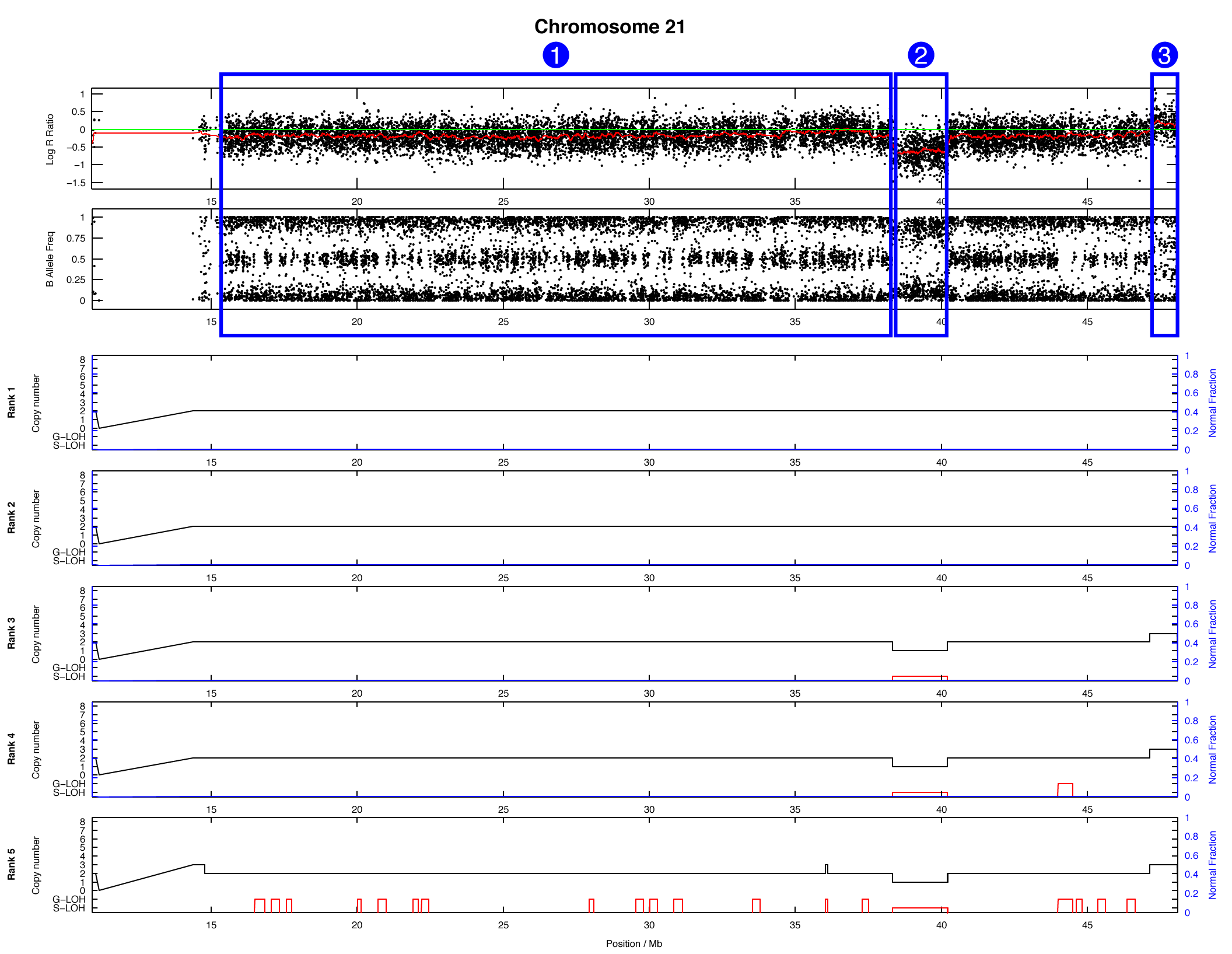
For each of the highlighted regions (1), (2), and (3) try to identify: (a) the number of copies present, (b) whether loss-of-heterozygosity has occurred, and (c) what the major and minor allele counts are. We will take this opportunity to stop and discuss as a group.
Answers can be found here.
Part 2: Analysis of CNAs using Sequencing Data
The workflow for analyzing CNAs using sequencing data is not dramatically different from microarrays. The major difference is that we start with aligned sequencing reads in the form of .bam files, rather than raw microarray data in the form of .cel files.
We will use exome data from the same publicly available breast cancer cell line that we examined in the microarray section. This time we will also be making use of exome data from a matched normal sample. Note that this matched normal sample did not come directly from a patient, but from a lymphoblastoid cell line derived from the patient.
Processing sequencing data takes time, so several of the preprocessing steps have been completed for you. Detailed preprocessing instructions are available on the wiki, so you can reproduce this in your own time.
The raw sequencing data has been downloaded and aligned for you. This data should already be in the linked data directory you created:
ls $CNA_WORKSPACE/data/HCC1395/exome
Step 1 - Extract Binned Read Counts
While array analysis involved probe intensities, sequencing analysis uses binned read counts to infer copy number. We used the HMMcopy C package to extract the number of reads in each bin for 1000 bp bins across the genome, from both the tumour and normal .bam files. Please refer to the preprocessing wiki page for details, and try to reproduce this in your own time. For now, let’s create an analysis directory for this step, and copy the processed data into it:
mkdir -p $CNA_WORKSPACE/analysis/exome/hmmcopy
cd $CNA_WORKSPACE/analysis/exome/hmmcopy
cp /home/ubuntu/CourseData/CG_data/Module6/analysis/exome/hmmcopy/* $CNA_WORKSPACE/analysis/exome/hmmcopy
The output is in the form of .wig files for the tumour and normal. These files specify the number of reads that fall into each genomic bin. The format is not very human-friendly, but you can take a look:
less -S HCC1395_exome_tumour.wig
fixedStep chrom=1 start=1 step=1000 span=1000
0
0
0
0
0
0
0
0
0
0
4
131
2489
364
5161
2013
8030
15030
9189
2672
9082
Step 2 - Identify Heterozygous SNPs and Extract Allele Counts
The next step in CNA analysis for sequencing data is to identify heterozygous germline variants from the matched normal genome, and use those positions to extract b-allele frequencies (BAF) from the tumour genome.
This step has also been completed for you using MutationSeq. Please refer to the preprocessing wiki page for details, and try to reproduce this in your own time. Let’s create an analysis directory for this step, and copy that data:
mkdir -p $CNA_WORKSPACE/analysis/exome/mutationseq
cd $CNA_WORKSPACE/analysis/exome/mutationseq
cp /home/ubuntu/CourseData/CG_data/Module6/analysis/exome/mutationseq/* $CNA_WORKSPACE/analysis/exome/mutationseq
The file HCC1395_mutationseq.vcf contains the raw output of MutationSeq, which was run in single-sample mode on the normal exome. This output was processed using a custom script to produce the format needed for Titan. Let’s take a look at the processed data:
column -t HCC1395_mutationseq_postprocess_filtered.txt | less -S
| chr | position | ref | refCount | Nref | NrefCount |
|---|---|---|---|---|---|
| 20 | 126529 | G | 5 | X | 5 |
| 20 | 138179 | C | 3 | X | 6 |
| 20 | 168466 | T | 37 | X | 32 |
| 20 | 171627 | G | 2 | X | 2 |
| 20 | 207889 | G | 39 | X | 47 |
| 20 | 210061 | G | 65 | X | 98 |
Step 3 - Generate Reference GC Content and Mappability Files
In order to correct the binned read counts for GC bias and mappability, we need to generate files based on the reference genome. Once again, this step has been completed for you using the HMMcopy C package, but details can be found in the preprocessing wiki page.
The two files that were generated for you in this step are the GC content file and mappability file, which you can find in the ref_data directory:
ls $CNA_WORKSPACE/ref_data/*.wig
Homo_sapiens.GRCh37.75.dna.primary_assembly.gc.wig
Homo_sapiens.GRCh37.75.dna.primary_assembly.fa.map.ws_1000.wig
Note that if you want to use a different reference genome or a different bin size for your CNA analysis, you will need to generate new files specific to that reference and bin size.
Step 4 - Call CNAs with Titan
We are now ready to call copy number alterations with Titan, which is available as an R Bioconductor package (TitanCNA).
The Titan R package includes a set of functions you can use to carry out CNA analysis, rather than an executable which can be run from the command line. Because of this, an R script scripts/run_titan.R for running Titan has been provided for you. Please note that this script only allows you specify a few important Titan parameters from the command line. If you want more control over your analysis, you can consult the Titan manual and edit the R script.
Launch the analysis as follows:
mkdir -p $CNA_WORKSPACE/analysis/exome/titan
cd $CNA_WORKSPACE/analysis/exome/titan
Rscript $CNA_WORKSPACE/scripts/run_titan.R \
	--sample_id HCC1395 \
	--tumour_wig $CNA_WORKSPACE/analysis/exome/hmmcopy/HCC1395_exome_tumour.wig \
	--normal_wig $CNA_WORKSPACE/analysis/exome/hmmcopy/HCC1395_exome_normal.wig \
	--tumour_baf $CNA_WORKSPACE/analysis/exome/mutationseq/HCC1395_mutationseq_postprocess_filtered.txt \
	--gc_wig $CNA_WORKSPACE/ref_data/Homo_sapiens.GRCh37.75.dna.primary_assembly.gc.wig \
	--map_wig $CNA_WORKSPACE/ref_data/Homo_sapiens.GRCh37.75.dna.primary_assembly.fa.map.ws_1000.wig \
	--result_dir $CNA_WORKSPACE/analysis/exome/titan \
	--exome_bed $CNA_WORKSPACE/ref_data/NimbleGenExome_v3.bed \
	--num_clust 1 \
	--ploidy 2.0 \
	--normal_con 0.0 \
	> run_titan.log \
	2> run_titan.err &
Some important parameters to consider:
--exome_bed: Specify the location of a.bedfile with the exome capture regions. If you are running whole-genome analysis, see below for how to modify the R script.--num_clust: This will set the TitannumberClonalClustersparameter. Specify the number of copy number sub-clones in the sample. It is common to run Titan several times with different settings for this value (e.g. 1, 2, 3). Here we will run Titan assuming a single clonal population. Below, we will discuss how to choose between different cluster numbers for more complex samples.--ploidy: This will set the Titan$ploidyParams$phi_0parameter. Specify an initial estimate for the ploidy of the sample. Titan will try to estimate the ploidy, but the initial value setting can influence the results. You can run Titan with different ploidy settings (e.g. 2.0, 4.0) and let it converge, or you can turn ploidy estimation off within the R script and Titan will use the provided value.--normal_con: This will set the Titan$normalParams$n_0parameter. Specify an initial estimate for the normal cell contamination of the sample. Titan will try to estimate the normal cell contamination, or you can turn estimation off within the R script and Titan will use the provided value.
Note that the workflow for running Titan with whole-genome data is the same as running it on exome data. The only difference is that you don’t need to specify the capture region when doing whole-genome analysis. In the script we used, you would need to modify the following line:
cnData <- correctReadDepth(tumWig, normWig, gcWig, mapWig, genomeStyle = "NCBI", targetedSequence = exomeCaptureSpaceDf)
If you want to analyze the entire genome, simply remove the last parameter specifying the target region: targetedSequence = exomeCaptureSpaceDf. Everything else should be the same.
Now, just like the OncoSNP analysis, the & symbol will cause the job to run in the background. You can check the progress of the job with:
less -S run_titan.log
Press q to exit the less program when you are finished viewing the log. This will take a few minutes to run. Take this time to review the R script itself. Please ask any questions you may have regarding the content of the script:
less $CNA_WORKSPACE/scripts/run_titan.R
When the analysis is complete, this script will generate a copy number plot for each chromosome using the default functions provided in the Titan package. This requires X11 forwarding and may fail since we are working on a server. For demonstration purposes, the plots can be copied as follows:
cp /home/ubuntu/CourseData/CG_data/Module6/analysis/exome/titan/*.png $CNA_WORKSPACE/analysis/exome/titan
Finally, a Titan segment file and an IGV compatible .seg file can be generated using a Perl script:
perl $CNA_WORKSPACE/scripts/createTITANsegmentfiles.pl \
	-id=test \
	-infile=$CNA_WORKSPACE/analysis/exome/titan/HCC1395.titan_results.txt \
	-outfile=$CNA_WORKSPACE/analysis/exome/titan/HCC1395.titan_results.seg.txt \
	-outIGV=$CNA_WORKSPACE/analysis/exome/titan/HCC1395.titan_results.seg
The .seg files can be opened in IGV to compare multiple samples. See the IGV website for more details regarding the .seg format.
Understanding Titan Results
We would like to be able to identify copy number heterogeneity, and select between Titan runs with a different number of clonal clusters. The cell line data we have been using doesn’t have much in the way of heterogeneity, and we can’t upload patient data onto the servers, so while Titan is running let’s take a look at some figures from a patient dataset.
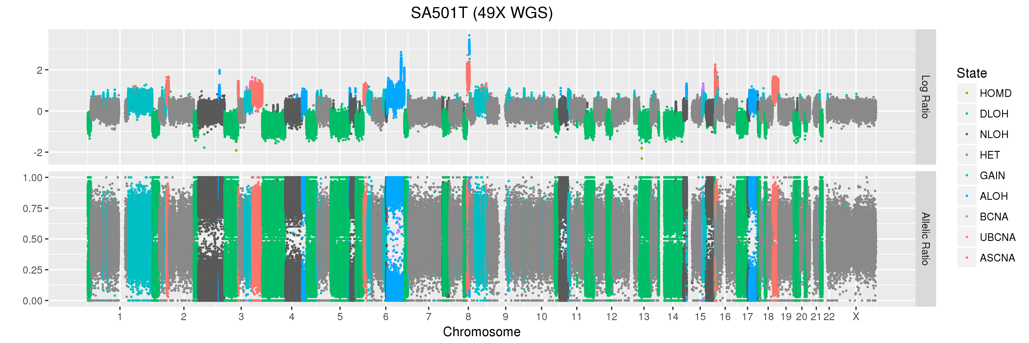
The copy number profiles we will be looking at come from a primary triple-negative breast cancer patient tumour (SA501T) sequenced as part of this study which looked at clonal dynamics in patient-derived xenografts.
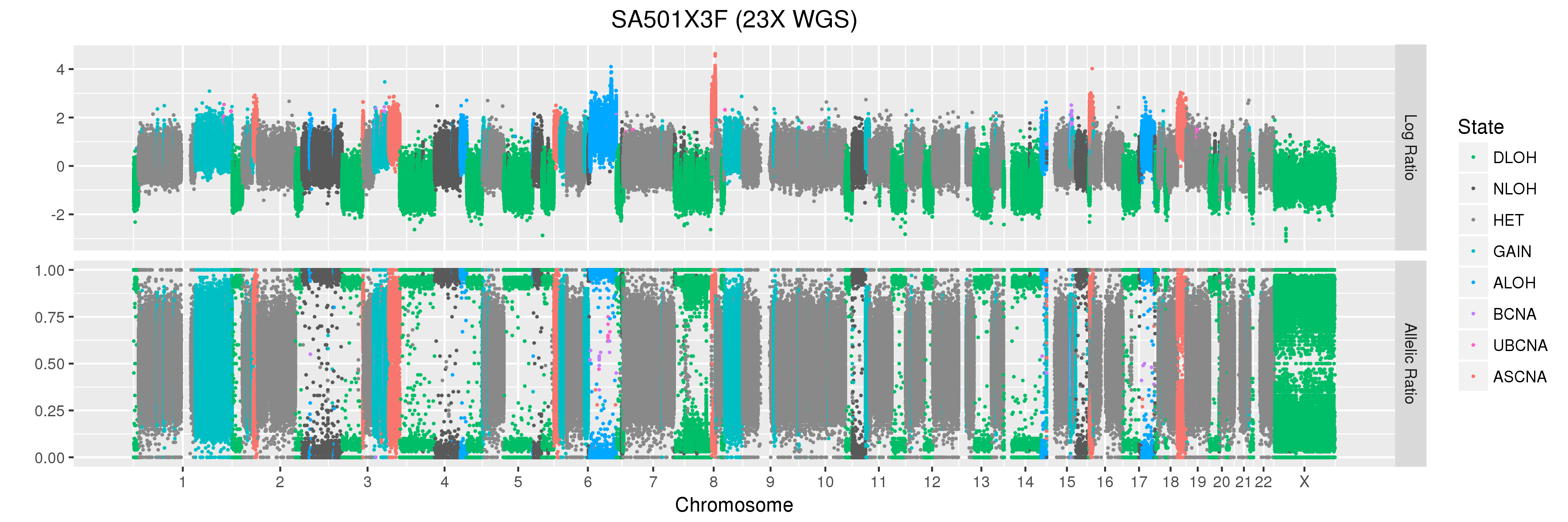
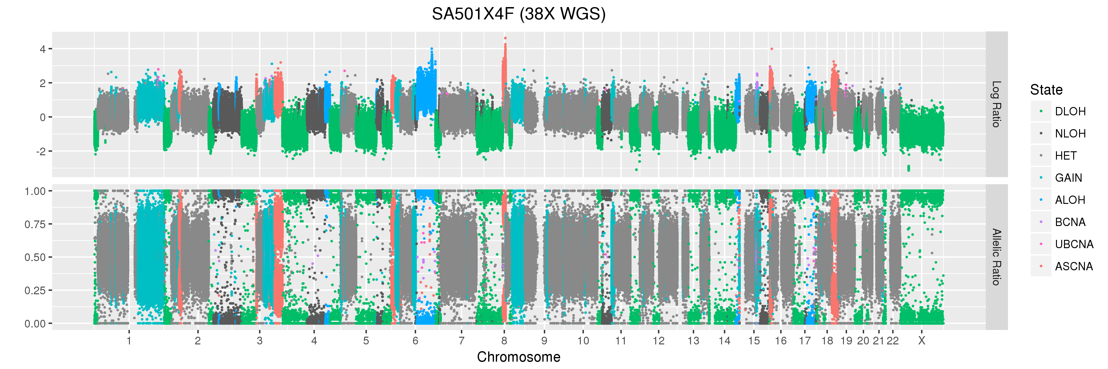
We will also look at Titan profiles from two xenograft passages derived from this patient: SA501X3F, a third-passage xenograft tumour; and SA501X4F, a fourth-passage xenograft tumour derived from SA501X3F.
Choosing the Number of Clusters
We ran Titan on the whole-genome .bam files from these three tumours, with three separate runs specifying either 1, 2, or 3 clonal clusters. You can copy the plots and parameter files as follows (actual Titan output is not provided to protect patient confidentiality):
cp /home/ubuntu/CourseData/CG_data/Module6/module6_cna_plots.zip $CNA_WORKSPACE
unzip module6_cna_plots.zip
You can then download the entire zip file or individual plots from your browser (XX is your student number):
http://##.oicrcbw.ca/Module6/module4_cna_plots
Titan uses the expectation-maximization (EM) algorithm to find the most likely values of the parameters. When given a more complex model (i.e. more clusters), this approach can over-fit and assign higher likelihood to runs with more clusters. So in order to choose the number of clusters, it is recommended not just to look at the likelihood, but at the DBW validity index which Titan provides at the end of the parameter file (lower index values are better):
less $CNA_WORKSPACE/module4_cna_plots/SA501/SA501T-49X/SA501T-49X_cluster1_params.txt
Normal contamination estimate:	0.26
Average tumour ploidy estimate:	1.88
Clonal cluster cellular prevalence Z=1:	0.9974
Genotype binomial means for clonal cluster Z=1:	0.50 0.79 0.87 0.54 0.90 0.63 0.92 0.71 0.54 0.94 0.76 0.59 0.95 0.80 0.65 0.50 0.95 0.82 0.69 0.56 0.96 0.84 0.73 0.61 0.55
Genotype Gaussian means for clonal cluster Z=1:	-1.84 -0.59 0.07 0.07 0.52 0.52 0.86 0.86 0.86 1.14 1.14 1.14 1.37 1.37 1.37 1.37 1.57 1.57 1.57 1.57 1.74 1.74 1.74 1.74 1.74
Genotype Gaussian variance:	0.0013 0.0139 0.0124 0.0124 0.0103 0.0103 0.0079 0.0079 0.0079 0.0044 0.0044 0.0044 0.0016 0.0016 0.0016 0.0016 0.0141 0.0141 0.0141 0.0141 0.0015 0.0015 0.0015 0.0015 0.0015
Number of iterations:	6
Log likelihood:	-2839305.1566
S_Dbw dens.bw (LogRatio):	0.0050
S_Dbw scat (LogRatio):	0.0163
S_Dbw validity index (LogRatio):	0.0213
S_Dbw dens.bw (AllelicRatio):	0.0062
S_Dbw scat (AllelicRatio):	0.0142
S_Dbw validity index (AllelicRatio):	0.0204
S_Dbw dens.bw (Both):	0.0112
S_Dbw scat (Both):	0.0305
S_Dbw validity index (Both):	0.0417
We summarized the results of the three runs with different cluster numbers in the optimal clusters file:
less $CNA_WORKSPACE/module4_cna_plots/SA501/SA501T-49X/SA501T-49X_titan_optimal_clusters.txt
case: SA501T num_clusters: 1 Ploidy: 1.88 DBW validity index: 0.0417
case: SA501T num_clusters: 2 Ploidy: 1.88 DBW validity index: 0.0585
case: SA501T num_clusters: 3 Ploidy: 1.88 DBW validity index: 0.0585

optimal Clusters: (1, '1.88')
optimal DBW index: 0.0417
********************************************************************************
You can see that Titan predicts one major copy number population in this patient tumour sample.
Now take a look at the summary file for the xenograft tumour SA501X3F:
less $CNA_WORKSPACE/module4_cna_plots/SA501/SA501X3F-23X/SA501X3F-23X_titan_optimal_clusters.txt
case: SA501X3F num_clusters: 1 Ploidy: 1.79 DBW validity index: 0.0843
case: SA501X3F num_clusters: 2 Ploidy: 1.79 DBW validity index: 0.0725
case: SA501X3F num_clusters: 3 Ploidy: 1.79 DBW validity index: 0.076

optimal Clusters: (2, '1.79')
optimal DBW index: 0.0725
********************************************************************************
Titan predicts that this sample has two major copy number clones. For SA501X4F, Titan also predicts a single major copy number clone. We will use the results from these runs in the question section below.
Questions
Question 1
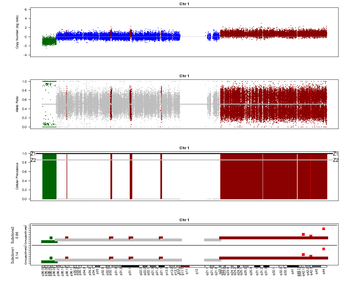
Let’s take a look at the chromosome 1 Titan plots from SA501X3F cluster2 and SA501X4F cluster1.
SA501X3F (whole-genome sequencing at 23X depth), chromosome 1:
SA501X4F (whole-genome sequencing at 38X depth), chromosome 1:
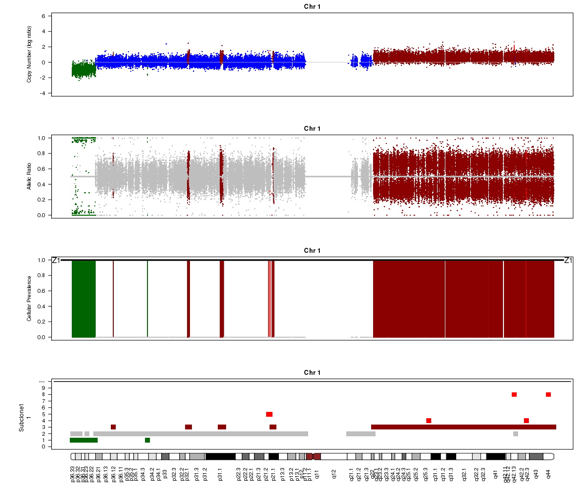
Take a look at the allelic ratio values in the heterozygous region - they are slightly more “spread out” in SA501X3F than SA501X4F. Why might this be?
Question 2
Now let’s compare the chromosome 1 results for SA501X4F (above) with the patient tumour SA501T cluster 1.
SA501T (whole-genome sequencing at 49X depth), chromosome 1:
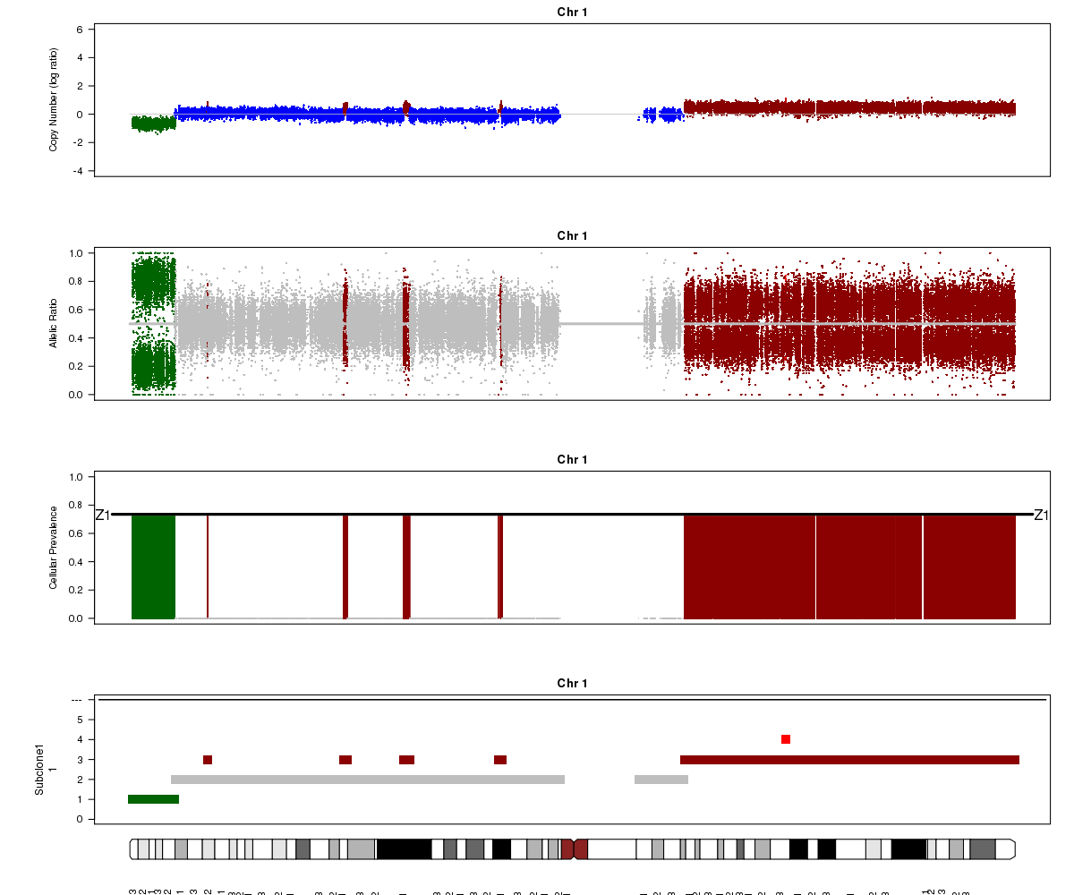
Notice the allelic ratio values in the deleted region are “shifted inwards” in the tumour sample, whereas they are at 0 or 1 in the xenograft. Why might this be?
Question 3
Look again at the SA501T plot above. What is Titan’s normal contamination estimate?
Question 4
Now look again at the SA501X3F plot above. What is Titan’s estimated prevalence for the two clones?
Question 5
The bottom track in the SA501X3F plot (see Question 1) shows the predicted profiles for the two clones. Notice that for chromosome 1, the profiles are the same for the two clones. Browse through all of the chromosomes for SA501X3F cluster 2. In which chromosomes are the two clones predicted to have differences in copy number?
Note that it is not only the lowest plot that is different, but that the “Cellular Prevalence” plot (third track) also indicates differences between clonal populations.
Question 6
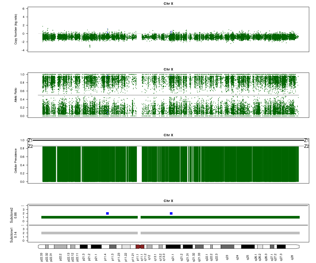
Now let’s look at chromosome X in all three of the samples. What is going on here?
SA501T (whole-genome sequencing at 49X depth), chromosome X:
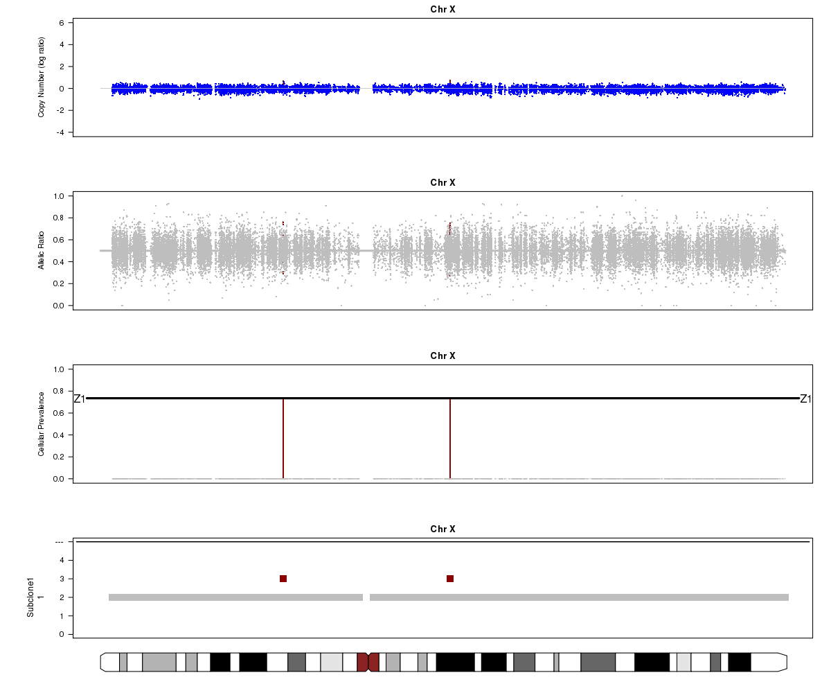
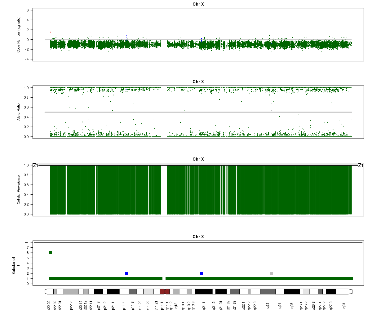
SA501X3F (whole-genome sequencing at 23X depth), chromosome X:
SA501X4F (whole-genome sequencing at 38X depth), chromosome X:
Answers:
(1) SA501X3F was sequenced at lower depth which makes the BAF values more noisy.
(2) SA501T has normal cell contamination. Titan looks at BAF values in the tumour for positions that are heterozygous in the normal, so if normal cells are present, they will shift the BAF values towards 0.5.
(3) About 25%. See the “Z1” line in the “Cellular Prevalence” plot. Of course, a more precise value can be found in the parameter file (26%).
(4) About 85% and 15% based on the “Z2” line in the “Cellular Prevalence” plot. The bottom “Subclone” plot actually shows the estimated values (86% and 14%).
(5) Chromosome X.
(6) A sub-clone with only one copy of chromosome X emerges and becomes dominant over time. The original patient tumour SA501T has one major population, which has 2 copies of chromosome X. In the third-passage xenograft SA501X3F, most of the population has lost one copy of X, leading to loss-of-heterozygosity and an “outward” shift in BAF values. Only a minor population (about 15%) of cells with 2 copies of chromosome X remain. By the fourth-passage SA501X4F, the ancestral population with two copies of X is no longer detectable, and Titan predicts one major population with a single copy of X.
Troubleshooting
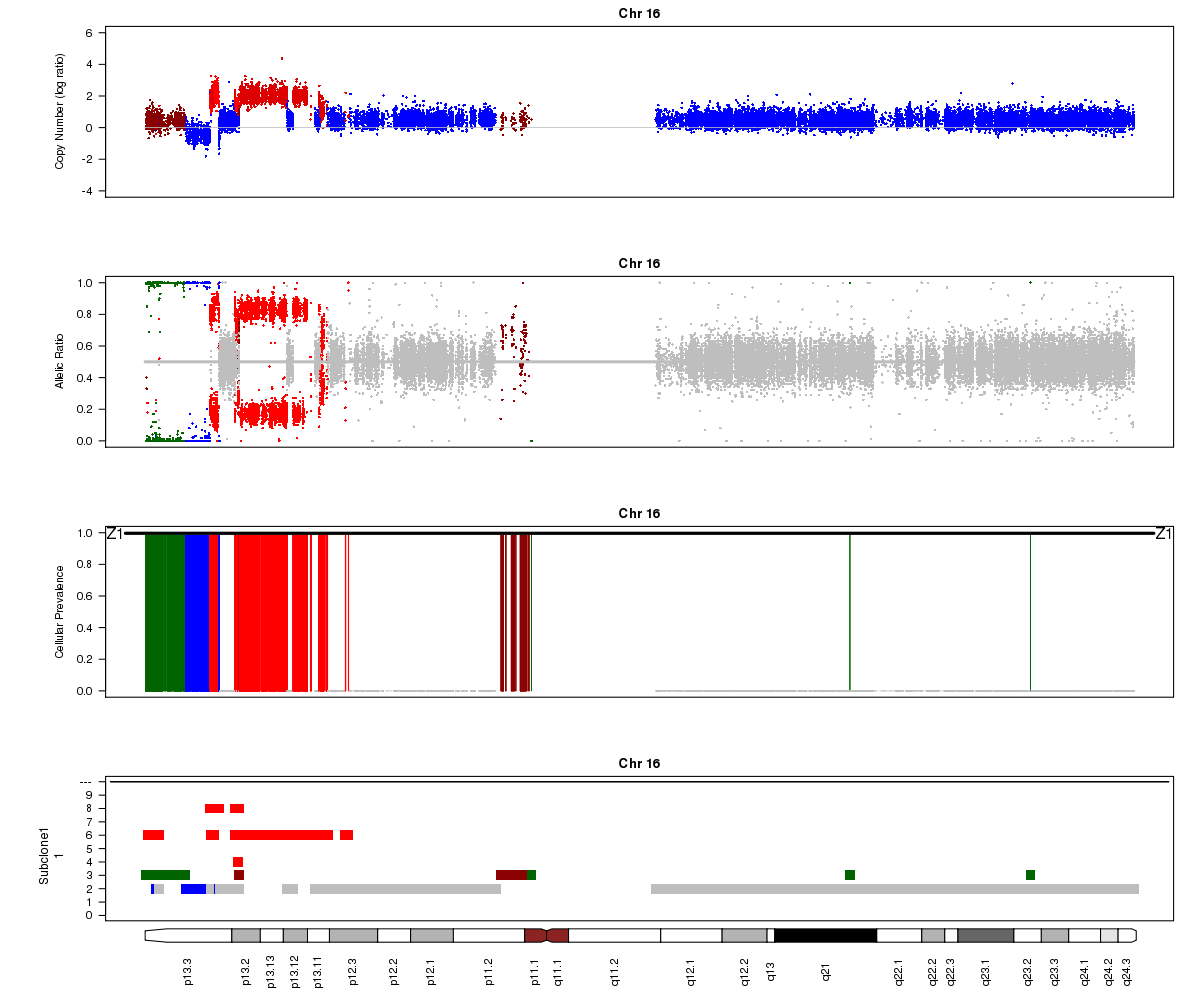
Titan may sometimes converge to a local rather than global maximum solution. In the example below from SA501X3F, Titan converged to the wrong ploidy value, resulting in strange state assignments. Can you point out segments in this plot that indicate the calls are incorrect? Hint: look at the colours assigned to different regions in the LRR plot.
SA501X3F chromosome 16, ploidy converged to 2.50:
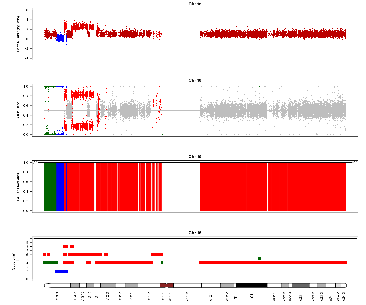
Titan may also sometimes converge to two ploidy values, one of which is twice the other (e.g. 2.0 and 4.0). In this case, the solution is unidentifiable. In the example below for SA501X3F (whose true ploidy of approximately 1.8 has been experimentally confirmed), the Titan result of approximately 3.6 is equally logical. Note that you will not see any regions assigned to the 1-copy DLOH state in this case:
SA501X3F chromosome 16, ploidy converged to 3.56:
Below is another example from a different sample where the Titan results don’t seem to make sense (image courtesy of Andrew McPherson). Can you guess what went wrong? Hint: it isn’t Titan’s fault this time!
Patient 15 chromosome 10 (cluster 3):
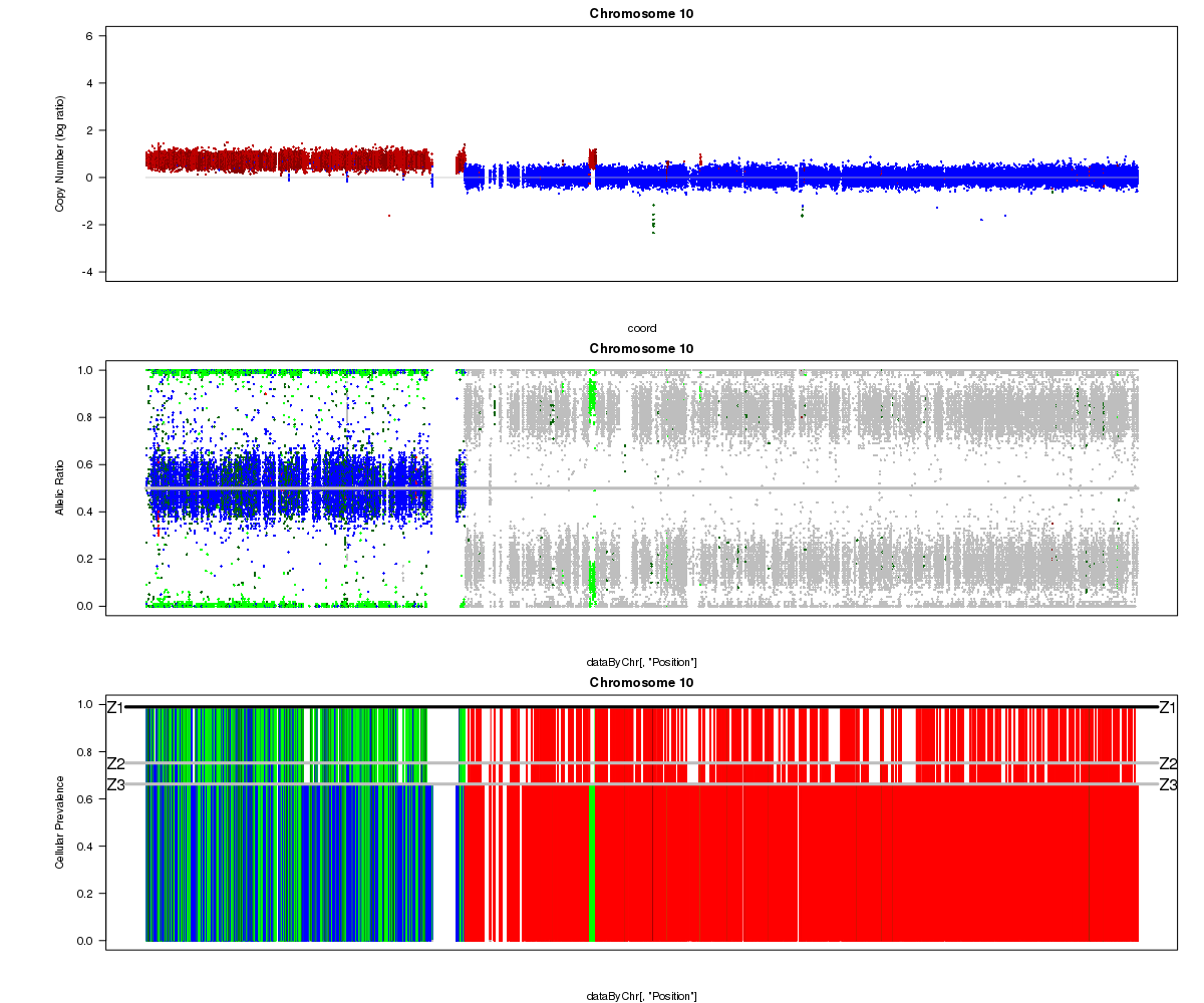
Answer: the “matched normal” sample used in the analysis was not actually from the same patient as the tumour. You can see the correct profile after the mismatch was resolved here.
Plotting with R
We can use a programming language like R to further explore the Titan results. For example, the default Titan functions plot each chromosome separately, and we may want to visualize the entire genome. The plots also don’t have a legend, and we may want to customize the colours used for the different states for easier interpretation. To do this, we will use the popular R package ggplot2. We’ll first copy the relevant scripts for plotting our figures into our titan folder.
Let’s start an RStudio instance by opening the web browser and entering:
http://XX.oicrcbw.ca:8080
Where the XX is your student number. Now click on the Console, and run this to set the working directory:
setwd("/home/ubuntu/workspace/Module6/analysis/exome/titan")
Setting the working directory allows us to open and write files in a particular location without specifying the full path. In general, using relative rather than absolute paths is not a good idea, since it makes the code harder to transfer to others. However, for the sake of this tutorial we will do this for convenience.
Now you have two options. The first option is to open the R script plot_titan.R and run it line-by-line (you can copy and paste the lines into the console, or press control-Enter to execute the line of code where your cursor is currently placed). The plots will then appear in the “Plots” tab on the right.
The second option is to open the R markdown file plot_titan.Rmd. This contains the same code and annotations, but it can be run interactively by clicking the green Play button next to each chunk of code. The plots will then appear in-line. These markdown files can be exported (complete with code, plots, and annotations) to other formats such as PDF, HTML, or Word.
Go to File -> Open File and choose the file you want to work with. Please feel free to ask for help as you go.
Interpretation
Details of the Titan state calls can be found in the Supplement of the Titan paper (Supplementary Table 14). A simplified summary is below:
| Titan Call | Definition |
|---|---|
| HOMD | Homozygous deletion |
| DLOH | Hemizygous deletion LOH |
| NLOH | Copy neutral LOH |
| HET | Heterozygous diploid |
| GAIN | One-copy gain |
| ALOH | Amplification LOH |
| BCNA | Balanced copy number amplification |
| UBCNA | Unbalanced copy number amplification |
| ASCNA | Allele-specific copy number amplification |
Finally, let’s take a look at the whole-genome plots for SA501T, SA501X3F, and SA501X4F.
For SA501X3F, you can clearly see that the BAF values for chromosome X are “shifted inwards” relative to the BAF values for other regions that Titan called DLOH. This is a clear indication of copy number heterogeneity.