Informatics for RNA-Seq Analysis
De novo RNA-Seq Assembly, Annotation, and Analysis Using Trinity and Trinotate
The following details the steps involved in:
- Generating a Trinity de novo RNA-Seq assembly
- Quantifying transcript expression levels
- Identifying differentially expressed (DE) transcripts
- Functionally annotating transcripts using Trinotate and predicting coding regions using TransDecoder
- Examining functional enrichments for DE transcripts using GOseq
- Interactively Exploring annotations and expression data via TrinotateWeb
Setting up your environment
Before we begin, set up your environment like so:
% source ~/CourseData/RNA_data/trinity_trinotate_tutorial_2018/environment.txt
Create your workspace
% mkdir ~/workspace/trinity_and_trinotate

% cd ~/workspace/trinity_and_trinotate
Data Content:
For this course we will be using the data from this paper: Defining the transcriptomic landscape of Candida glabrata by RNA-Seq. Linde et al. Nucleic Acids Res. 2015 This work provides a detailed RNA-Seq-based analysis of the transcriptomic landscape of C. glabrata in nutrient-rich media (WT), as well as under nitrosative stress (GSNO), in addition to other conditions, but we’ll restrict ourselves to just WT and GSNO conditions for demonstration purposes in this workshop.
There are paired-end FASTQ formatted Illlumina read files for each of the two conditions, with three biological replicates for each.
Copy all these data to your workspace like so:
% cp -r ~/CourseData/RNA_data/trinity_trinotate_tutorial_2018/C_glabrata data
All RNA-Seq data sets can be found in the data/ subdirectory:
% ls -1 data/* | grep fastq
.
GSNO_SRR1582646_1.fastq
GSNO_SRR1582646_2.fastq
GSNO_SRR1582647_1.fastq
GSNO_SRR1582647_2.fastq
GSNO_SRR1582648_1.fastq
GSNO_SRR1582648_2.fastq
wt_SRR1582649_1.fastq
wt_SRR1582649_2.fastq
wt_SRR1582650_1.fastq
wt_SRR1582650_2.fastq
wt_SRR1582651_1.fastq
wt_SRR1582651_2.fastq
Each biological replicate (eg. wt_SRR1582651) contains a pair of fastq files (eg. wt_SRR1582651_1.fastq.gz for the ‘left’ and wt_SRR1582651_2.fastq.gz for the ‘right’ read of the paired end sequences). Normally, each file would contain millions of reads, but in order to reduce running times as part of the workshop, each file provided here is restricted to only 10k RNA-Seq reads.
It’s generally good to evaluate the quality of your input data using a tool such as FASTQC. Since exploration of FASTQC reports has already been done in a previous section of this workshop, we’ll skip doing it again here - and trust that the quality of these reads meet expectations.
Finally, another set of files that you will find in the data include ‘mini_sprot.pep*’, corresponding to a highly abridged version of the SWISSPROT database, containing only the subset of protein sequences that are needed for use in this workshop. It’s provided and used here only to speed up certain operations, such as BLAST searches, which will be performed at several steps in the tutorial below. Of course, in exploring your own RNA-Seq data, you would leverage the full version of SWISSPROT and not this tiny subset used here.
De novo assembly of reads using Trinity
To generate a reference assembly that we can later use for analyzing differential expression, we’ll combine the read data sets for the different conditions together into a single target for Trinity assembly. We do this by providing Trinity with a list of the targeted fastq files organized according to sample type and replicate name, as provided in a ‘samples.txt’ file.
Take a look at the samples.txt file:
% cat data/samples.txt
.
 GSNO    GSNO_SRR1582646 data/GSNO_SRR1582646_1.fastq    data/GSNO_SRR1582646_2.fastq
 GSNO    GSNO_SRR1582647 data/GSNO_SRR1582647_1.fastq    data/GSNO_SRR1582647_2.fastq
 GSNO    GSNO_SRR1582648 data/GSNO_SRR1582648_1.fastq    data/GSNO_SRR1582648_2.fastq
 wt      wt_SRR1582649   data/wt_SRR1582649_1.fastq      data/wt_SRR1582649_2.fastq
 wt      wt_SRR1582650   data/wt_SRR1582650_1.fastq      data/wt_SRR1582650_2.fastq
 wt      wt_SRR1582651   data/wt_SRR1582651_1.fastq      data/wt_SRR1582651_2.fastq
Using this samples.txt file, perform de novo transcriptome assembly of the reads with Trinity like so:
%   ${TRINITY_HOME}/Trinity --seqType fq  --samples_file data/samples.txt \
      --CPU 2 --max_memory 2G --min_contig_length 150
Running Trinity on this data set may take 10 to 15 minutes. You’ll see it progress through the various stages, starting with Jellyfish to generate the k-mer catalog, then followed by Inchworm to assemble ‘draft’ contigs, Chrysalis to cluster the contigs and build de Bruijn graphs, and finally Butterfly for tracing paths through the graphs and reconstructing the final isoform sequences.
Running a typical Trinity job requires ~1 hour and ~1G RAM per ~1 million PE reads. You’d normally run it on a high-memory machine and let it churn for hours or days.
The assembled transcripts will be found at ‘trinity_out_dir/Trinity.fasta’.
Just to look at the top few lines of the assembled transcript fasta file, you can run:
% head trinity_out_dir/Trinity.fasta
and you can see the Fasta-formatted Trinity output:
>TRINITY_DN506_c0_g1_i1 len=171 path=[149:0-170] [-1, 149, -2]
TGAGTATGGTTTTGCCGGTTTGGCTGTTGGTGCAGCTTTGAAGGGCCTAAAGCCAATTGT
TGAATTCATGTCATTCAACTTCTCCATGCAAGCCATTGACCATGTCGTTAACTCGGCAGC
AAAGACACATTATATGTCTGGTGGTACCCAAAAATGTCAAATCGTGTTCAG
>TRINITY_DN512_c0_g1_i1 len=168 path=[291:0-167] [-1, 291, -2]
ATATCAGCATTAGACAAAAGATTGTAAAGGATGGCATTAGGTGGTCGAAGTTTCAGGTCT
AAGAAACAGCAACTAGCATATGACAGGAGTTTTGCAGGCCGGTATCAGAAATTGCTGAGT
AAGAACCCATTCATATTCTTTGGACTCCCGTTTTGTGGAATGGTGGTG
>TRINITY_DN538_c0_g1_i1 len=310 path=[575:0-309] [-1, 575, -2]
GTTTTCCTCTGCGATCAAATCGTCAAACCTTAGACCTAGCTTGCGGTAACCAGAGTACTT
Note, the sequences you see will likely be different, as the order of sequences in the output is not deterministic.
The FASTA sequence header for each of the transcripts contains the identifier for the transcript (eg. ‘TRINITY_DN506_c0_g1_i1’), the length of the transcript, and then some information about how the path was reconstructed by the software by traversing nodes within the graph.
It is often the case that multiple isoforms will be reconstructed for the same ‘gene’. Here, the ‘gene’ identifier corresponds to the prefix of the transcript identifier, such as ‘TRINITY_DN506_c0_g1’, and the different isoforms for that ‘gene’ will contain different isoform numbers in the suffix of the identifier (eg. TRINITY_DN506_c0_g1_i1 and TRINITY_DN506_c0_g1_i2 would be two different isoform sequences reconstructed for the single gene TRINITY_DN506_c0_g1). It is useful to perform certain downstream analyses, such as differential expression, at both the ‘gene’ and at the ‘isoform’ level, as we’ll do later below.
Evaluating the assembly
There are several ways to quantitatively as well as qualitatively assess the overall quality of the assembly, and we outline many of these methods at our Trinity wiki.
For the sake of time, we’re going to skip this as part for now.
Transcript expression quantitation using Salmon
To estimate transcript expression values, we’ll use the salmon software. We’ll run salmon on each of the sample replicates as listed in our samples.txt file:
%  $TRINITY_HOME/util/align_and_estimate_abundance.pl --seqType fq  \
    --samples_file data/samples.txt  --transcripts trinity_out_dir/Trinity.fasta \
    --est_method salmon  --trinity_mode   --prep_reference
The above should have generated separate sets of outputs for each of the sample replicates. Examine the new contents of your working directory:
% ls -ltr
.
...
drwxr-xr-x   9 bhaas  1594166068     306 Jan  5 18:19 wt_SRR1582651
drwxr-xr-x   9 bhaas  1594166068     306 Jan  5 18:21 GSNO_SRR1582646
drwxr-xr-x   9 bhaas  1594166068     306 Jan  5 18:21 GSNO_SRR1582648
drwxr-xr-x   9 bhaas  1594166068     306 Jan  5 18:21 GSNO_SRR1582647
drwxr-xr-x   9 bhaas  1594166068     306 Jan  5 18:21 wt_SRR1582650
drwxr-xr-x   9 bhaas  1594166068     306 Jan  5 18:21 wt_SRR1582649
Take a look at the contents of one of these salmon output directories:
% ls -ltr wt_SRR1582651
.
drwxr-xr-x  3 bhaas  1594166068    102 Jan  5 18:19 logs
drwxr-xr-x  3 bhaas  1594166068    102 Jan  5 18:19 libParams
drwxr-xr-x  8 bhaas  1594166068    272 Jan  5 18:19 aux_info
-rw-r--r--  1 bhaas  1594166068  30752 Jan  5 18:21 quant.sf.genes
-rw-r--r--  1 bhaas  1594166068  30181 Jan  5 18:21 quant.sf
-rw-r--r--  1 bhaas  1594166068    631 Jan  5 18:21 lib_format_counts.json
-rw-r--r--  1 bhaas  1594166068    432 Jan  5 18:21 cmd_info.json
Examine the contents of the ‘quant.sf’ file:
% head wt_SRR1582651/quant.sf | column -t
.
Name                   Length  EffectiveLength  TPM      NumReads
TRINITY_DN0_c0_g1_i1   308     157.95           1965.28  9
TRINITY_DN1_c0_g1_i1   240     96.0038          2155.59  6
TRINITY_DN10_c0_g1_i1  473     319.649          539.512  5
TRINITY_DN11_c0_g1_i1  416     262.791          1181.23  9
TRINITY_DN12_c0_g1_i1  362     209.731          1151.17  7
TRINITY_DN14_c0_g1_i1  174     43.8077          787.324  1
TRINITY_DN14_c0_g2_i1  277     128.996          534.759  2
TRINITY_DN15_c0_g1_i1  172     42.4787          811.956  1
TRINITY_DN15_c0_g2_i1  309     158.847          434.264  2
The key columns in the above salmon output are the transcript identifier ‘Name’, the ‘NumReads’ corresponding to the number of RNA-Seq fragments predicted to be derived from that transcript, and the ‘TPM’ column indicates the normalized expression values for the expression of that transcript in the sample (measured as Transcripts Per Million).
Generate a transcript counts matrix and perform cross-sample normalization:
Now, given the expression estimates for each of the transcripts in each of the samples, we’re going to pull together all values into matrices containing transcript IDs in the rows, and sample names in the columns. We’ll make two matrices, one containing the estimated counts, and another containing the TPM expression values that are cross-sample normalized using the TMM method. This is all done for you by the following script in Trinity, indicating the method we used for expresssion estimation and providing the list of individual sample abundance estimate files.
First, let’s create a list of the quant.sf files:
% find wt_* GSNO_* -name "quant.sf" | tee quant_files.list
.
 wt_SRR1582649/quant.sf
 wt_SRR1582650/quant.sf
 wt_SRR1582651/quant.sf
 GSNO_SRR1582646/quant.sf
 GSNO_SRR1582647/quant.sf
 GSNO_SRR1582648/quant.sf
Using this new file ‘quant_files.list’, we’ll use a Trinity script to generate the count and expression matrices for both the transcript isoforms and sepearate files for ‘gene’s.
% $TRINITY_HOME/util/abundance_estimates_to_matrix.pl --est_method salmon \
--out_prefix Trinity --name_sample_by_basedir \
--quant_files quant_files.list \
--gene_trans_map trinity_out_dir/Trinity.fasta.gene_trans_map
You should find a matrix file called ‘Trinity.isoform.counts.matrix’, which contains the counts of RNA-Seq fragments mapped to each transcript.
Examine the first few lines of the counts matrix:
% head -n20 Trinity.isoform.counts.matrix | column -t
.
                     wt_SRR1582649           wt_SRR1582650  wt_SRR1582651  GSNO_SRR1582646  GSNO_SRR1582647  GSNO_SRR1582648
     TRINITY_DN543_c0_g1_i1  0              4              1                1                2                0
     TRINITY_DN256_c0_g3_i1  13             5              8                0                1                0
     TRINITY_DN288_c0_g3_i1  29             20             22               0                0                0
     TRINITY_DN596_c0_g1_i1  1              1              1                2                3                0
     TRINITY_DN353_c0_g1_i1  3              0              0                1                1                2
     TRINITY_DN260_c0_g2_i1  0              0              1                2                6                2
     TRINITY_DN235_c0_g1_i2  3              0              4                8                15               9.30823
     TRINITY_DN276_c0_g2_i1  26             17             30               2                4                2
     TRINITY_DN527_c0_g1_i1  4              4              4                28               34               29
You’ll see that the above matrix has integer values representing the number of RNA-Seq paired-end fragments that are estimated to have been derived from that corresponding transcript in each of the samples. Don’t be surprised if you see some values that are not exact integers but rather fractional read counts. This happens if there are multiply-mapped reads (such as to common sequence regions of different isoforms), in which case the multiply-mapped reads are fractionally assigned to the corresponding transcripts according to their maximum likelihood.
The counts matrix will be used by DESeq2 (or other tools in Bioconductor) for statistical analysis and identifying significantly differentially expressed transcripts.
Now take a look at the first few lines of the normalized expression matrix:
% head -n20 Trinity.isoform.TMM.EXPR.matrix | column -t
.
        wt_SRR1582649           wt_SRR1582650  wt_SRR1582651  GSNO_SRR1582646  GSNO_SRR1582647  GSNO_SRR1582648
TRINITY_DN543_c0_g1_i1  0.000          4285.916       1207.919         1250.354         2318.497         0.000
TRINITY_DN256_c0_g3_i1  2882.375       1075.231       1763.201         0.000            219.023          0.000
TRINITY_DN288_c0_g3_i1  2429.634       1634.889       1688.699         0.000            0.000            0.000
TRINITY_DN596_c0_g1_i1  1083.186       1009.491       1133.029         2358.738         3293.404         0.000
TRINITY_DN353_c0_g1_i1  2738.546       0.000          0.000            994.050          930.488          2204.007
TRINITY_DN260_c0_g2_i1  0.000          0.000          721.127          1501.711         4235.108         1677.503
TRINITY_DN235_c0_g1_i2  365.070        0.000          457.735          980.110          1779.601         1347.575
TRINITY_DN276_c0_g2_i1  1690.132       1078.912       1764.242         129.311          251.891          154.163
TRINITY_DN527_c0_g1_i1  313.156        305.603        285.846          2186.494         2582.453         2694.495
These are the normalized expression values, which have been further cross-sample normalized using TMM normalization to adjust for any differences in sample composition. TMM normalization assumes that most transcripts are not differentially expressed, and linearly scales the expression values of samples to better enforce this property. TMM normalization is described in A scaling normalization method for differential expression analysis of RNA-Seq data, Robinson and Oshlack, Genome Biology 2010.
We use the TMM-normalized expression matrix when plotting expression values in heatmaps and other expression analyses.
Note, similar count and expression files were generated at the ‘gene’ level as well, and these can be used similarly to the isoform matrices wherever you want to perform a gene-based analysis instead. It’s often useful to study the expression data at both the gene and isoform level, particularly in cases where differential transcript usage exists (isoform switching), where differences in expression may not be apparent at the gene level.
Differential Expression Using DESeq2
A plethora of tools are currently available for identifying differentially expressed transcripts based on RNA-Seq data, and of these, DESeq2 is among the most popular and most accurate. The DESeq2 software is part of the R Bioconductor package, and we provide support for using it in the Trinity package.
Having biological replicates for each of your samples is crucial for accurate detection of differentially expressed transcripts. In our data set, we have three biological replicates for each of our conditions, and in general, having three or more replicates for each experimental condition is highly recommended.
To detect differentially expressed transcripts, run the Bioconductor package DESeq2 using our counts matrix:
%  $TRINITY_HOME/Analysis/DifferentialExpression/run_DE_analysis.pl \
      --matrix Trinity.isoform.counts.matrix \
      --samples_file data/samples.txt \
      --method DESeq2 \
      --output DESeq2_trans
Examine the contents of the DESeq2_trans/ directory.
% ls -ltr DESeq2_trans/
.
-rw-r--r--  1 bhaas  1594166068    1545 Jan  5 23:56 Trinity.isoform.counts.matrix.GSNO_vs_wt.DESeq2.Rscript
-rw-r--r--  1 bhaas  1594166068   24550 Jan  5 23:57 Trinity.isoform.counts.matrix.GSNO_vs_wt.DESeq2.count_matrix
-rw-r--r--  1 bhaas  1594166068   15522 Jan  5 23:57 Trinity.isoform.counts.matrix.GSNO_vs_wt.DESeq2.DE_results.MA_n_Volcano.pdf
-rw-r--r--  1 bhaas  1594166068  115612 Jan  5 23:57 Trinity.isoform.counts.matrix.GSNO_vs_wt.DESeq2.DE_results
The files ‘*.DE_results’ contain the output from running DESeq2 to identify differentially expressed transcripts in each of the pairwise sample comparisons. Examine the format of one of the files, such as the results from comparing Sp_log to Sp_plat:
% head DESeq2_trans/Trinity.isoform.counts.matrix.GSNO_vs_wt.DESeq2.DE_results | column -t
.
                      sampleA                 sampleB  baseMeanA  baseMeanB         baseMean          log2FoldChange    lfcSE              stat               pvalue             padj
TRINITY_DN486_c0_g1_i1  GSNO     wt         16.8981745355167  106.980365419029  61.9392699772726  -2.6493893326134   0.255388975436606  -10.3739377476419  3.25815666078611e-25  1.7384467428526e-22
TRINITY_DN577_c0_g1_i1  GSNO     wt         15.7288302868206  101.644075065183  58.6864526760018  -2.69899406362077  0.261493095561904  -10.3214735280911  5.63515962026775e-25  1.7384467428526e-22
TRINITY_DN556_c0_g1_i1  GSNO     wt         23.9663919729509  105.796343729641  64.8813678512961  -2.15116963920305  0.233191735883499  -9.2248965472677   2.83834758240544e-20  5.8375348611472e-18
TRINITY_DN324_c0_g1_i1  GSNO     wt         1.47231222746358  80.2499964184142  40.8611543229389  -5.79076278854971  0.677003202157668  -8.55352348422289  1.19386992588915e-17  1.84154436068402e-15
TRINITY_DN310_c0_g1_i1  GSNO     wt         1.93665704962814  64.4895090163414  33.2130830329848  -4.99435027412214  0.588931323085661  -8.48036108515101  2.24496126493146e-17  2.77028220092542e-15
TRINITY_DN157_c0_g2_i1  GSNO     wt         53.21625596387    4.41363265791558  28.8149443108928  3.59667509622987   0.4743359674083    7.58254769479438   3.38834460951473e-14  3.48434770678431e-12
TRINITY_DN142_c0_g1_i1  GSNO     wt         0                 64.3364882003275  32.1682441001638  -8.65066949183313  1.19947555120541   -7.21204319932964  5.5118480566932e-13   4.55603207727768e-11
TRINITY_DN143_c0_g1_i1  GSNO     wt         1.10944933305853  52.0143601526098  26.5619047428341  -5.49448910934864  0.762847590122535  -7.20260400700233  5.90733494622713e-13  4.55603207727768e-11
TRINITY_DN601_c0_g1_i1  GSNO     wt         71.5561235105584  16.9551033864134  44.2556134484859  2.06065562273661   0.293266276985126  7.02656863216878   2.11674484549853e-12  1.45114618852511e-10
These data include the log fold change (log2FoldChange), mean expression (baseMean), P- value from an exact test, and false discovery rate (padj).
The DESeq2 analysis above generated both MA and Volcano plots based on these data. Examine any of these, such as ‘DESeq2_trans/Trinity.isoform.counts.matrix.GSNO_vs_wt.DESeq2.DE_results.MA_n_Volcano.pdf’ from within your web browser.

The red data points correspond to all those features that were identified as being significant with an FDR <= 0.05.
Trinity facilitates analysis of these data, including scripts for extracting transcripts that are above some statistical significance (FDR threshold) and fold-change in expression, and generating figures such as heatmaps and other useful plots, as described below.
Extracting differentially expressed transcripts and generating heatmaps
Now let’s perform the following operations from within the DESeq2_trans/ directory. Enter the DESeq2_trans/ dir like so:
% cd DESeq2_trans/
Extract those differentially expressed (DE) transcripts that are at least 4-fold differentially expressed at a significance of <= 0.001 in any of the pairwise sample comparisons:
% $TRINITY_HOME/Analysis/DifferentialExpression/analyze_diff_expr.pl \
      --matrix ../Trinity.isoform.TMM.EXPR.matrix \
      --samples ../data/samples.txt \
      -P 1e-3 -C 2
The above generates several output files with a prefix diffExpr.P1e-3_C2’, indicating the parameters chosen for filtering, where P (FDR actually) is set to 0.001, and fold change (C) is set to 2^(2) or 4-fold. (These are default parameters for the above script. See script usage before applying to your data).
Included among these files are: ‘diffExpr.P1e-3_C2.matrix’ : the subset of the FPKM matrix corresponding to the DE transcripts identified at this threshold. The number of DE transcripts identified at the specified thresholds can be obtained by examining the number of lines in this file.
% wc -l diffExpr.P1e-3_C2.matrix
.
(n) diffExpr.P1e-3_C2.matrix
where n ~ 100 to 110
Note, the number of lines in this file includes the top line with column names, so there are actually (n-1) DE transcripts at this 4-fold and 1e-3 FDR threshold cutoff.
Also included among these files is a heatmap ‘diffExpr.P1e-3_C2.matrix.log2.centered.genes_vs_samples_heatmap.pdf’ as shown below, with transcripts clustered along the vertical axis and samples clustered along the horizontal axis.
View file ‘diffExpr.P1e-3_C2.matrix.log2.centered.genes_vs_samples_heatmap.pdf’ from within your web browser.
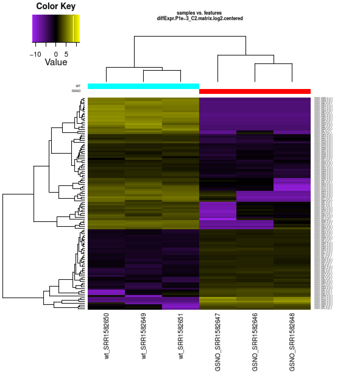
The expression values are plotted in log2 space and mean-centered (mean expression value for each feature is subtracted from each of its expression values in that row), and shows upregulated expression as yellow and downregulated expression as purple.
Extract transcript clusters by expression profile by cutting the dendrogram
Extract clusters of transcripts with similar expression profiles by cutting the transcript cluster dendrogram at a given percent of its height (ex. 60%), like so:
% $TRINITY_HOME/Analysis/DifferentialExpression/define_clusters_by_cutting_tree.pl \
       --Ptree 60 -R diffExpr.P1e-3_C2.matrix.RData
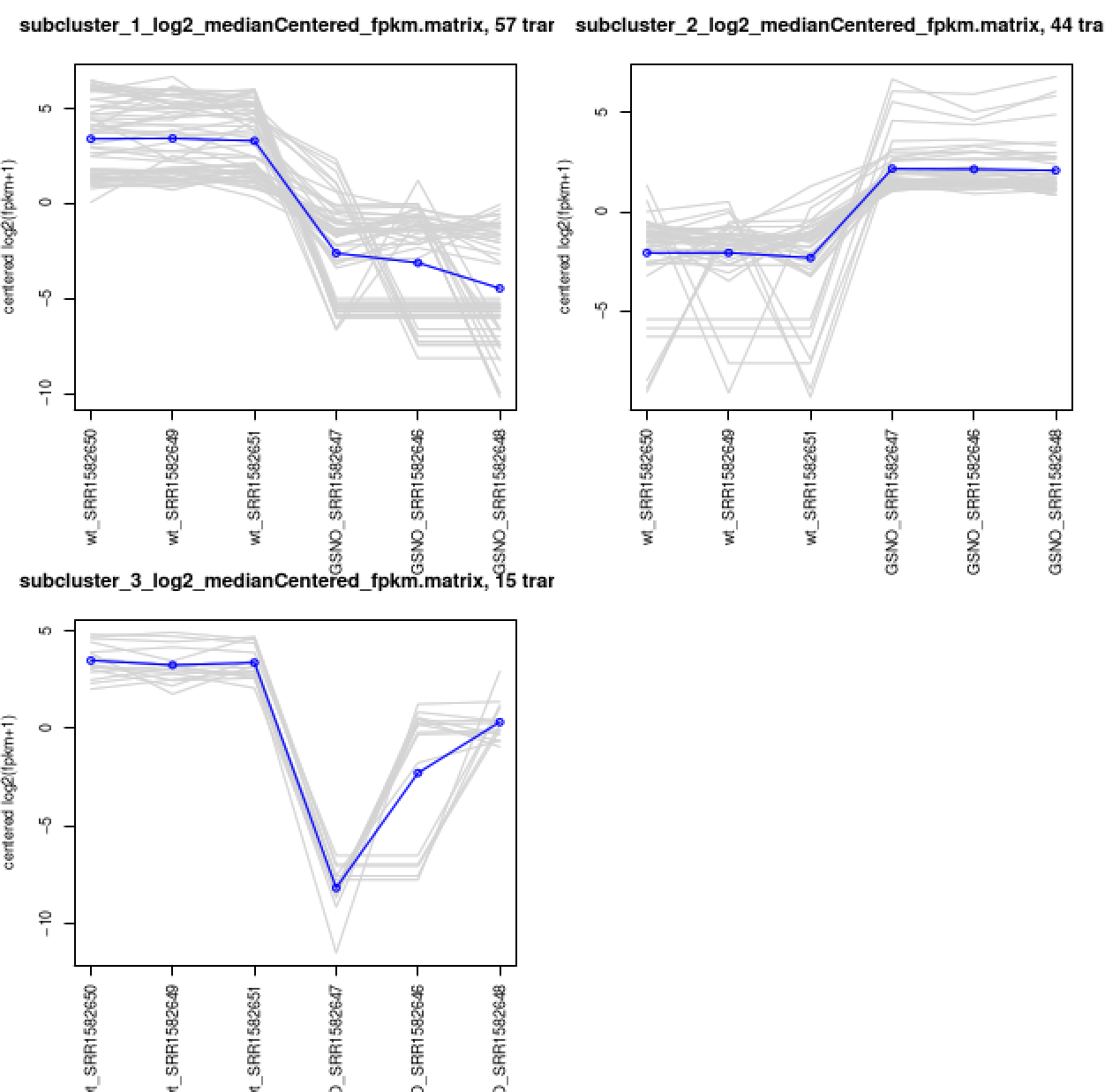
This creates a directory containing the individual transcript clusters, including a pdf file that summarizes expression values for each cluster according to individual charts:
View file ‘diffExpr.P1e-3_C2.matrix.RData.clusters_fixed_P_60/my_cluster_plots.pdf’ from your web browser.
Rinse & repeat: DE analysis at the gene level
You can do all the same analyses as you did above at the gene level. For now, let’s just rerun the DE detection step, since we’ll need the results later on for use with TrinotateWeb. Also, it doesn’t help us to study the ‘gene’ level data with this tiny data set (yet another disclaimer) given that all our transcripts = genes, since we didn’t find any alternative splicing variants. With typical data sets, you will have alterantively spliced isoforms identified, and performing DE analysis at the gene level should provide more power for detection than at the isoform level. For more info about this, I encourage you to read this paper.
Before running the gene-level DE analysis, be sure to back out of the current DESeq2_trans/ directory like so:
% cd ../
Be sure you’re in your base working directory:
% pwd
.
/home/ubuntu/workspace/trinity_and_trinotate
Now, run the DE analysis at the gene level like so:
%  $TRINITY_HOME/Analysis/DifferentialExpression/run_DE_analysis.pl \
      --matrix Trinity.gene.counts.matrix \
      --samples_file data/samples.txt \
      --method DESeq2 \
      --output DESeq2_gene
You’ll now notice that the DESeq2_gene/ directory exists and is populated with similar files.
% ls -ltr DESeq2_gene/
Let’s move on and make use of those outputs later. With your own data, however, you would normally run the same set of operations as you did above for the transcript-level DE analyses.
Functional Annotation of Assembled Transcripts Using Trinotate
Now we have a bunch of transcript sequences and have identified some subset of them that appear to be biologically interesting in that they’re differentially expressed between our two conditions - but we don’t really know what they are or what biological functions they might represent. We can explore their potential functions by functionally annotating them using our Trinotate software and analysis protocol. To learn more about Trinotate, you can visit the Trinotate website.
Again, let’s make sure that we’re back in our primary working directory called ‘trinity_and_trinotate’:
% pwd
.
/home/ubuntu/workspace/trinity_and_trinotate
If you’re not in the above directory, then relocate yourself to it.
Now, create a Trinotate/ directory and relocate to it. We’ll use this as our Trinotate computation workspace.
% mkdir Trinotate

% cd Trinotate
Bioinformatics analyses to gather evidence for potential biological functions
Below, we’re going to run a number of different tools to capture information about our transcript sequences.
Identification of likely protein-coding regions in transcripts
TransDecoder is a tool we built to identify likely coding regions within transcript sequences. It identifies long open reading frames (ORFs) within transcripts and scores them according to their sequence composition. Those ORFs that encode sequences with compositional properties (codon frequencies) consistent with coding transcripts are reported.
Running TransDecoder is a two-step process. First run the TransDecoder step that identifies all long ORFs.
% $TRANSDECODER_HOME/TransDecoder.LongOrfs -t ../trinity_out_dir/Trinity.fasta
Now, run the step that predicts which ORFs are likely to be coding.
% $TRANSDECODER_HOME/TransDecoder.Predict -t ../trinity_out_dir/Trinity.fasta
You’ll now find a number of output files containing ‘transdecoder’ in their name:
% ls -1 |grep transdecoder
.
Trinity.fasta.transdecoder.bed
Trinity.fasta.transdecoder.cds
Trinity.fasta.transdecoder.gff3
Trinity.fasta.transdecoder.pep
Trinity.fasta.transdecoder_dir/
...
The file we care about the most here is the ‘Trinity.fasta.transdecoder.pep’ file, which contains the protein sequences corresponding to the predicted coding regions within the transcripts.
Go ahead and take a look at this file:
% less Trinity.fasta.transdecoder.pep
.
>TRINITY_DN107_c0_g1_i1.p1 TRINITY_DN107_c0_g1~~TRINITY_DN107_c0_g1_i1.p1  ORF type:internal len:175 (+),score=164.12 TRINITY_DN107_c0_g1_i1:2-523(+)
VPLYQHLADLSDSKTSPFVLPVPFLNVLNGGSHAGGALALQEFMIAPTGAKSFREAMRIG
SEVYHNLKSLTKKRYGSSAGNVGDEGGVAPDIQTAEEALDLIVDAIKAAGHEGKVKIGLD
CASSEFFKDGKYDLDFKNPNSDASKWLSGPQLADLYHSLVKKYPIVSIEDPFAE
>TRINITY_DN10_c0_g1_i1.p2 TRINITY_DN10_c0_g1~~TRINITY_DN10_c0_g1_i1.p2  ORF type:internal len:158 (-),score=122.60 TRINITY_DN10_c0_g1_i1:2-472(-)
TDQDKRYQAKMGKSHGYRSRTRYMFQRDFRKHGAIALSTYLKVYKVGDIVDIKANGSIQK
GMPHKFYQGKTGVVYNVTKSSVGVIVNKMVGNRYLEKRLNLRVEHVKHSKCRQEFLDRVK
SNAAKRAEAKAQGKAVQLKRQPAQPREARVVSTEGNV
>TRINITY_DN110_c0_g1_i1.p2 TRINITY_DN110_c0_g1~~TRINITY_DN110_c0_g1_i1.p2  ORF type:complete len:131 (+),score=98.69 TRINITY_DN110_c0_g1_i1:55-447(+)
MTRSSVLADALNAINNAEKTGKRQVLIRPSSKVIIKFLQVMQRHGYIGEFEYIDDHRSGK
Type ‘q’ to exit the ‘less’ viewer.
| There are a few items to take notice of in the above peptide file. The header lines includes the protein identifier composed of the original transcripts along with ‘ | m.(number)’. The ‘type’ attribute indicates whether the protein is ‘complete’, containing a start and a stop codon; ‘5prime_partial’, meaning it’s missing a start codon and presumably part of the N-terminus; ‘3prime_partial’, meaning it’s missing the stop codon and presumably part of the C-terminus; or ‘internal’, meaning it’s both 5prime-partial and 3prime-partial. You’ll also see an indicator (+) or (-) to indicate which strand the coding region is found on, along with the coordinates of the ORF in that transcript sequence. |
This .pep file will be used for various sequence homology and other bioinformatics analyses below.
Sequence homology searches
Earlier, we ran blastx against our mini SWISSPROT datbase to identify likely full-length transcripts. Let’s run blastx again to capture likely homolog information, and we’ll lower our E-value threshold to 1e-5 to be less stringent than earlier.
% blastx -db ../data/mini_sprot.pep \
         -query ../trinity_out_dir/Trinity.fasta -num_threads 2 \
         -max_target_seqs 1 -outfmt 6 -evalue 1e-5 \
          > swissprot.blastx.outfmt6
Now, let’s look for sequence homologies by just searching our predicted protein sequences rather than using the entire transcript as a target:
% blastp -query Trinity.fasta.transdecoder.pep \
         -db ../data/mini_sprot.pep -num_threads 2 \
         -max_target_seqs 1 -outfmt 6 -evalue 1e-5 \
          > swissprot.blastp.outfmt6
Using our predicted protein sequences, let’s also run a HMMER search against the Pfam database, and identify conserved domains that might be indicative or suggestive of function:
% hmmscan --cpu 2 --domtblout TrinotatePFAM.out \
          ../data/trinotate_data/Pfam-A.hmm \
          Trinity.fasta.transdecoder.pep
Note, hmmscan might take a few minutes to run.
Computational prediction of sequence features
The signalP and tmhmm software tools are very useful for predicting signal peptides (secretion signals) and transmembrane domains, respectively.
To predict signal peptides, run signalP like so:
% signalp -f short -n signalp.out Trinity.fasta.transdecoder.pep
Take a look at the output file:
% less signalp.out
.
##gff-version 2
##sequence-name source  feature start   end     score   N/A ?
## -----------------------------------------------------------
TRINITY_DN19_c0_g1_i1|m.141     SignalP-4.0     SIGNAL  1       18      0.553   .       .       YES
TRINITY_DN33_c0_g1_i1|m.174     SignalP-4.0     SIGNAL  1       19      0.631   .       .       YES
....
How many of your proteins are predicted to encode signal peptides?
Preparing and Generating a Trinotate Annotation Report
Generating a Trinotate annotation report involves first loading all of our bioinformatics computational results into a Trinotate SQLite database. The Trinotate software provides a boilerplate SQLite database called ‘Trinotate.sqlite’ that comes pre-populated with a lot of generic data about SWISSPROT records and Pfam domains (and is a pretty large file consuming several hundred MB). Below, we’ll populate this database with all of our bioinformatics computes and our expression data.
Preparing Trinotate (loading the database)
As a sanity check, be sure you’re currently located in your ‘Trinotate/’ working directory.
% pwd .

/home/ubuntu/workspace/trinity_and_trinotate/Trinotate
Copy the provided Trinotate.sqlite boilerplate database into your Trinotate working directory like so:
 %  cp ../data/trinotate_data/Trinotate.boilerplate.sqlite  Trinotate.sqlite

 %  chmod 644 Trinotate.sqlite  # make it writeable
Load your Trinotate.sqlite database with your Trinity transcripts and predicted protein sequences:
%  $TRINOTATE_HOME/Trinotate Trinotate.sqlite init \
     --gene_trans_map ../trinity_out_dir/Trinity.fasta.gene_trans_map \
     --transcript_fasta ../trinity_out_dir/Trinity.fasta \
     --transdecoder_pep Trinity.fasta.transdecoder.pep
Load in the various outputs generated earlier:
%  $TRINOTATE_HOME/Trinotate Trinotate.sqlite \
       LOAD_swissprot_blastx swissprot.blastx.outfmt6

%  $TRINOTATE_HOME/Trinotate Trinotate.sqlite \
       LOAD_swissprot_blastp swissprot.blastp.outfmt6

%  $TRINOTATE_HOME/Trinotate Trinotate.sqlite LOAD_pfam TrinotatePFAM.out

%  $TRINOTATE_HOME/Trinotate Trinotate.sqlite LOAD_signalp signalp.out
Generate the Trinotate Annotation Report
% $TRINOTATE_HOME/Trinotate Trinotate.sqlite report > Trinotate.xls
View the report
% less Trinotate.xls
.
#gene_id        transcript_id   sprot_Top_BLASTX_hit    TrEMBL_Top_BLASTX_hit   RNAMMER prot_id prot_coords     sprot_Top_BLASTP_hit    TrEMBL_Top_BLASTP_hit   Pfam    SignalP TmHMM   eggnog  gene_ontology_blast     gene_ontology_pfam      transcript      peptide
TRINITY_DN144_c0_g1     TRINITY_DN144_c0_g1_i1  PUT4_YEAST^PUT4_YEAST^Q:1-198,H:425-490^74.24%ID^E:4e-29^RecName: Full=Proline-specific permease;^Eukaryota; Fungi; Dikarya; Ascomycota; Saccharomycotina; Saccharomycetes; Saccharomycetales; Saccharomycetaceae; Saccharomyces        .       .       .       .
   .       .       .       .       .       COG0833^permease        GO:0016021^cellular_component^integral component of membrane`GO:0005886^cellular_component^plasma membrane`GO:0015193^molecular_function^L-proline transmembrane transporter activity`GO:0015175^molecular_function^neutral amino acid transmembrane transporter activity`GO:0015812^biological_process^gamma-aminobutyric acid transport`GO:0015804^biological_process^neutral amino acid transport`GO:0035524^biological_process^proline transmembrane transport`GO:0015824^biological_process^proline transport      .       .       .
TRINITY_DN179_c0_g1     TRINITY_DN179_c0_g1_i1  ASNS1_YEAST^ASNS1_YEAST^Q:1-168,H:158-213^82.14%ID^E:5e-30^RecName: Full=Asparagine synthetase [glutamine-hydrolyzing] 1;^Eukaryota; Fungi; Dikarya; Ascomycota; Saccharomycotina; Saccharomycetes; Saccharomycetales; Saccharomycetaceae; Saccharomyces        .
   .       .       .       .       .       .       .       .       COG0367^asparagine synthetase   GO:0004066^molecular_function^asparagine synthase (glutamine-hydrolyzing) activity`GO:0005524^molecular_function^ATP binding`GO:0006529^biological_process^asparagine biosynthetic process`GO:0006541^biological_process^glutamine metabolic process`GO:0070981^biological_process^L-asparagine biosynthetic process    .       .       .
TRINITY_DN159_c0_g1     TRINITY_DN159_c0_g1_i1  ENO2_CANGA^ENO2_CANGA^Q:2-523,H:128-301^100%ID^E:4e-126^RecName: Full=Enolase 2;^Eukaryota; Fungi; Dikarya; Ascomycota; Saccharomycotina; Saccharomycetes; Saccharomycetales; Saccharomycetaceae; Nakaseomyces; Nakaseomyces/Candida clade      .       .       TRINITY_DN159_c0_g1_i1|m.1      2-523[+]        ENO2_CANGA^ENO2_CANGA^Q:1-174,H:128-301^100%ID^E:3e-126^RecName: Full=Enolase 2;^Eukaryota; Fungi; Dikarya; Ascomycota; Saccharomycotina; Saccharomycetes; Saccharomycetales; Saccharomycetaceae; Nakaseomyces; Nakaseomyces/Candida clade      .       PF00113.17^Enolase_C^Enolase, C-terminal TIM barrel domain^18-174^E:9.2e-79     .       .       .       GO:0005829^cellular_component^cytosol`GO:0000015^cellular_component^phosphopyruvate hydratase complex`GO:0000287^molecular_function^magnesium ion binding`GO:0004634^molecular_function^phosphopyruvate hydratase activity`GO:0006096^biological_process^glycolytic process     GO:0000287^molecular_function^magnesium ion binding`GO:0004634^molecular_function^phosphopyruvate hydratase activity`GO:0006096^biological_process^glycolytic process`GO:0000015^cellular_component^phosphopyruvate hydratase complex   .       .
...
The above file can be very large. It’s often useful to load it into a spreadsheet software tools such as MS-Excel. If you have a transcript identifier of interest, you can always just ‘grep’ to pull out the annotation for that transcript from this report. We’ll use TrinotateWeb to interactively explore these data in a web browser below.
Let’s use the annotation attributes for the transcripts here as ‘names’ for the transcripts in the Trinotate database. This will be useful later when using the TrinotateWeb framework.
%  $TRINOTATE_HOME/util/annotation_importer/import_transcript_names.pl \
      Trinotate.sqlite Trinotate.xls
Nothing exciting to see in running the above command, but know that it’s helpful for later on.
Interactively Explore Expression and Annotations in TrinotateWeb
Earlier, we generated large sets of tab-delimited files containg lots of data - annotations for transcripts, matrices of expression values, lists of differentially expressed transcripts, etc. We also generated a number of plots in PDF format. These are all useful, but they’re not interactive and it’s often difficult and cumbersome to extract information of interest during a study. We’re developing TrinotateWeb as a web-based interactive system to solve some of these challenges. TrinotateWeb provides heatmaps and various plots of expression data, and includes search functions to quickly access information of interest. Below, we will populate some of the additional information that we need into our Trinotate database, and then run TrinotateWeb and start exploring our data in a web browser.
Populate the expression data into the Trinotate database
Once again, verify that you’re currently in the Trinotate/ working directory:
% pwd
.
/home/ubuntu/workspace/trinity_and_trinotate/Trinotate
Now, load in the transcript expression data stored in the matrices we built earlier:
%  $TRINOTATE_HOME/util/transcript_expression/import_expression_and_DE_results.pl \
        --sqlite Trinotate.sqlite \
        --transcript_mode \
        --samples_file ../data/samples.txt \
        --count_matrix ../Trinity.isoform.counts.matrix \
        --fpkm_matrix ../Trinity.isoform.TMM.EXPR.matrix
Import the DE results from our DESeq2_trans/ directory:
%  $TRINOTATE_HOME/util/transcript_expression/import_expression_and_DE_results.pl \
       --sqlite Trinotate.sqlite \
       --transcript_mode \
       --samples_file ../data/samples.txt \
       --DE_dir ../DESeq2_trans
and Import the clusters of transcripts we extracted earlier based on having similar expression profiles across samples:
%  $TRINOTATE_HOME/util/transcript_expression/import_transcript_clusters.pl \
       --sqlite Trinotate.sqlite \
       --group_name DE_all_vs_all \
       --analysis_name diffExpr.P1e-3_C2_clusters_fixed_P_60 \
        ../DESeq2_trans/diffExpr.P1e-3_C2.matrix.RData.clusters_fixed_P_60/*matrix
And now we’ll do the same for our gene-level expression and DE results:
%  $TRINOTATE_HOME/util/transcript_expression/import_expression_and_DE_results.pl \
        --sqlite Trinotate.sqlite \
        --gene_mode \
        --samples_file ../data/samples.txt \
        --count_matrix ../Trinity.gene.counts.matrix \
        --fpkm_matrix ../Trinity.gene.TMM.EXPR.matrix


%  $TRINOTATE_HOME/util/transcript_expression/import_expression_and_DE_results.pl \
       --sqlite Trinotate.sqlite \
       --gene_mode \
       --samples_file ../data/samples.txt \
       --DE_dir ../DESeq2_gene
Note, in the above gene-loading commands, the term ‘component’ is used. ‘Component’ is just another word for ‘gene’ in the realm of Trinity.
At this point, the Trinotate database should be fully populated and ready to be used by TrinotateWeb.
Launch and Surf TrinotateWeb
TrinotateWeb is web-based software and runs locally on the same hardware we’ve been running all our computes (as opposed to your typical websites that you visit regularly, such as facebook). Launch the mini webserver that drives the TrinotateWeb software like so:
% $TRINOTATE_HOME/run_TrinotateWebserver.pl 8080
Now, visit the following URL in Google Chrome: http://localhost:8080/cgi-bin/index.cgi
You should see a web form like so:
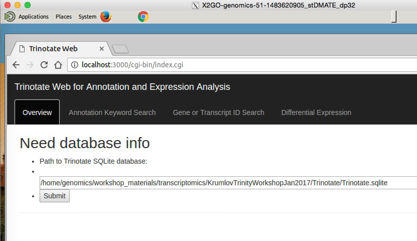
In the text box, put the path to your Trinotate.sqlite database, as shown above (“/home/ubuntu/workspace/trinity_and_trinotate/Trinotate/Trinotate.sqlite”). Click ‘Submit’.
You should now have TrinotateWeb running and serving the content in your Trinotate database:
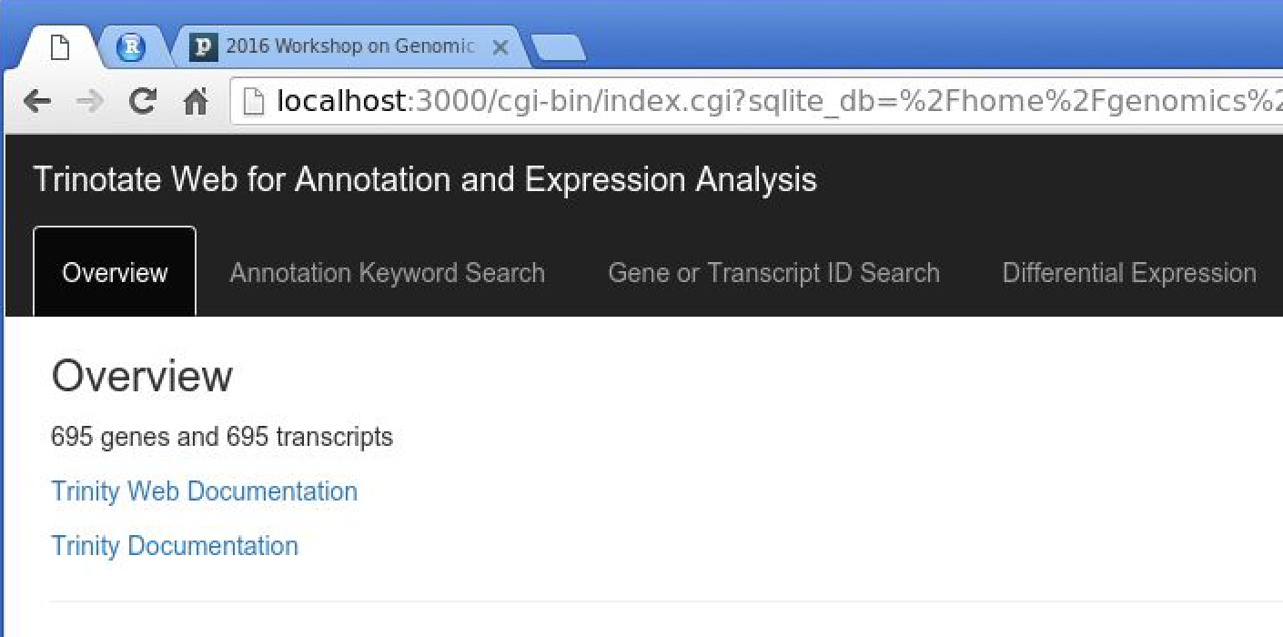
Take some time to click the various tabs and explore what’s available.
eg. Under ‘Annotation Keyword Search’, search for ‘transporter’
eg. Under ‘Differential Expression’, examine your earlier-defined transcript clusters. Also, launch MA or Volcano plots to explore the DE data.
We will explore TrinotateWeb functionality together as a group.
Epilogue
If you’ve gotten this far, hurray!!! Congratulations!!! You’ve now experienced the full tour of Trinity and TrinotateWeb. Visit our web documentation at http://trinityrnaseq.github.io, and join our Google group to become part of the ever-growing Trinity user community.