Module 1: Exploratory Data Analysis and Clustering

The goal of this lab is to examine correlation structure in a sample transcriptomic dataset using clustering.

We will start using a small mouse expression dataset from two tissues:

We will briefly explore the dataset using dim(), head(), and summary()
We will visualize correlation using pairs() and corrplot()
We will cluster samples using k-means and hierarchical clustering methods using dist() and hclust()
- We will assign samples to clusters using cutree() and visualize these using heatmap()
We will use clValid to find out what cluster number best separates groups

Finally we will explore clustering in a more complex bladder cancer dataset.

Load `mouse` data

For this exercise we are going to load a dataset built into the clValid package. This dataset measures 147 genes and expressed sequence tags in two developing mouse lineages: the neural crest cells and mesoderm-derived cells. There are three samples per group.

Let’s load the data.

suppressMessages(library(clValid))
data(mouse)

Use str() to see what types of data the columns have:

str(mouse)

## 'data.frame':    147 obs. of  8 variables:
##  $ ID : Factor w/ 147 levels "1415787_at","1415904_at",..: 111 88 93 74 138 103 46 114 112 24 ...
##  $ M1 : num  4.71 3.87 2.88 5.33 5.37 ...
##  $ M2 : num  4.53 4.05 3.38 5.5 4.55 ...
##  $ M3 : num  4.33 3.47 3.24 5.63 5.7 ...
##  $ NC1: num  5.57 5 3.88 6.8 6.41 ...
##  $ NC2: num  6.92 5.06 4.46 6.54 6.31 ...
##  $ NC3: num  7.35 5.18 4.85 6.62 6.2 ...
##  $ FC : Factor w/ 9 levels "ECM/Receptors",..: 3 8 6 6 1 3 1 6 5 6 ...

Another command is head():

head(mouse)

##             ID       M1       M2       M3      NC1      NC2      NC3                     FC
## 1   1448995_at 4.706812 4.528291 4.325836 5.568435 6.915079 7.353144 Growth/Differentiation
## 2 1436392_s_at 3.867962 4.052354 3.474651 4.995836 5.056199 5.183585   Transcription factor
## 3 1437434_a_at 2.875112 3.379619 3.239800 3.877053 4.459629 4.850978          Miscellaneous
## 4   1428922_at 5.326943 5.498930 5.629814 6.795194 6.535522 6.622577          Miscellaneous
## 5 1452671_s_at 5.370125 4.546810 5.704810 6.407555 6.310487 6.195847          ECM/Receptors
## 6   1448147_at 3.471347 4.129992 3.964431 4.474737 5.185631 5.177967 Growth/Differentiation

Summary provides useful information about the distribution of variables. Note that FC has categorical variables:

summary(mouse)

##           ID            M1              M2              M3             NC1             NC2       
##  1415787_at:  1   Min.   :2.352   Min.   :2.139   Min.   :2.500   Min.   :2.100   Min.   :1.996  
##  1415904_at:  1   1st Qu.:4.188   1st Qu.:4.151   1st Qu.:4.207   1st Qu.:4.174   1st Qu.:4.136  
##  1415993_at:  1   Median :4.994   Median :5.043   Median :5.054   Median :4.996   Median :5.056  
##  1416164_at:  1   Mean   :5.166   Mean   :5.140   Mean   :5.231   Mean   :5.120   Mean   :5.134  
##  1416181_at:  1   3rd Qu.:6.147   3rd Qu.:6.015   3rd Qu.:6.129   3rd Qu.:5.860   3rd Qu.:5.920  
##  1416221_at:  1   Max.   :9.282   Max.   :9.273   Max.   :9.228   Max.   :8.905   Max.   :8.954  
##  (Other)   :141                                                                                  
##       NC3                             FC    
##  Min.   :2.125   EST                   :31  
##  1st Qu.:4.293   Transcription factor  :28  
##  Median :4.974   Miscellaneous         :25  
##  Mean   :5.118   ECM/Receptors         :16  
##  3rd Qu.:5.826   Growth/Differentiation:16  
##  Max.   :9.251   Unknown               :10  
##                  (Other)               :21

What are the values in FC?

table(mouse$FC)

## 
##          ECM/Receptors                    EST Growth/Differentiation   Kinases/Phosphatases 
##                     16                     31                     16                      7 
##             Metabolism          Miscellaneous         Stress-induced   Transcription factor 
##                      8                     25                      6                     28 
##                Unknown 
##                     10

Usually the information about samples (“metadata”) is in a different table.

Let’s load the sample information about the mouse dataset:

pheno <- read.delim("AUR2024_data/mouse_pheno.txt",sep="\t",h=T,as.is=T)

Let’s look at it:

head(pheno)

##   SampleID         Type
## 1       M1  Mesenchymal
## 2       M2  Mesenchymal
## 3       M3  Mesenchymal
## 4      NC1 Neural-crest
## 5      NC2 Neural-crest
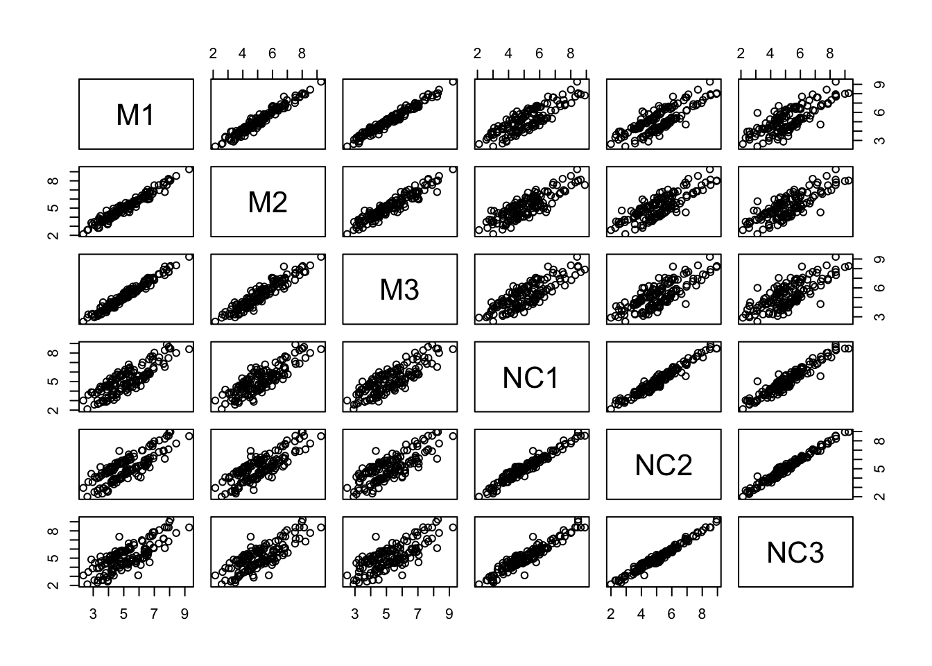
## 6      NC3 Neural-crest

Let’s use pairs() to look at pairwise scatterplots of the expression data in a single plot. We need to subset the columns with the expression data first:

mouse_exp = mouse[,c("M1","M2","M3","NC1","NC2","NC3")]
pairs(mouse_exp)

Correlations, distances, and clustering

Let’s look at sample correlation matrix. This should be a square matrix, equal to the number of samples. We have six samples, so the correlation matrix should be 6x6.

library(corrplot)

## corrplot 0.95 loaded

mouse_cor <- cor(mouse_exp)
dim(mouse_cor)

## [1] 6 6

round(mouse_cor,2)

##       M1   M2   M3  NC1  NC2  NC3
## M1  1.00 0.98 0.98 0.84 0.81 0.78
## M2  0.98 1.00 0.95 0.84 0.81 0.79
## M3  0.98 0.95 1.00 0.82 0.78 0.75
## NC1 0.84 0.84 0.82 1.00 0.97 0.95
## NC2 0.81 0.81 0.78 0.97 1.00 0.99
## NC3 0.78 0.79 0.75 0.95 0.99 1.00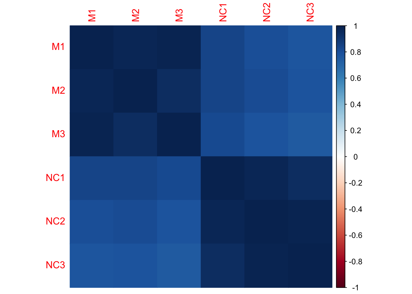

corrplot(mouse_cor, method="color")

Which samples appear to be best correlated with each other?
Which samples don’t appear to be as well correlated with each other?

Hierarchical clustering

Hierarchical clustering requires distances between samples. Let’s use dist() to compute these distances, and hclust() to generate the hierarchical clustering object.

d <- dist(t(log(mouse_exp)))

Using these distances, we cluster the samples using hierarchical clustering:

h <- hclust(d,method="ward.D2")

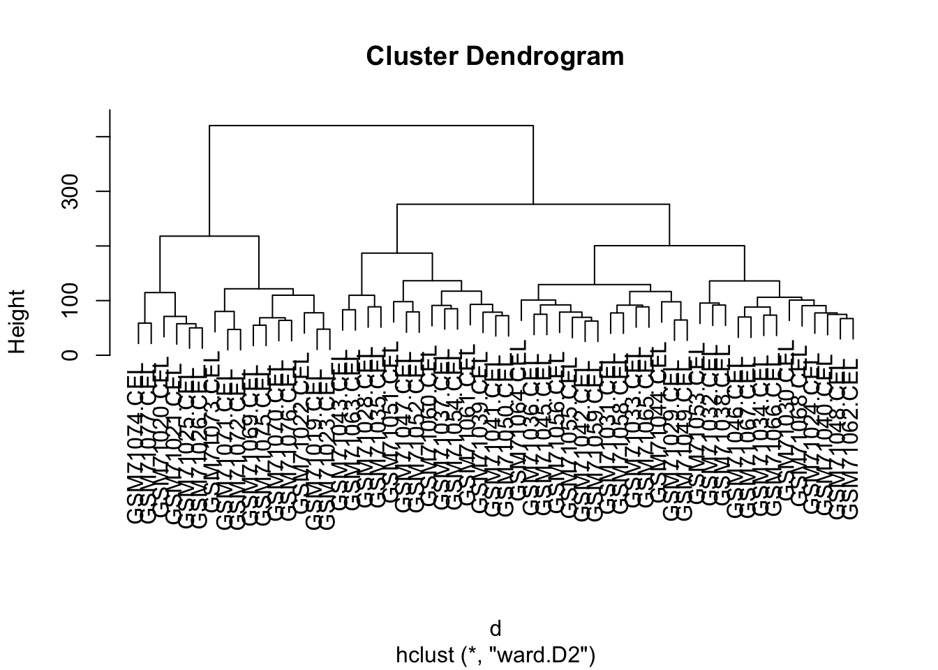
The output of this can be plotted:

plot(h)

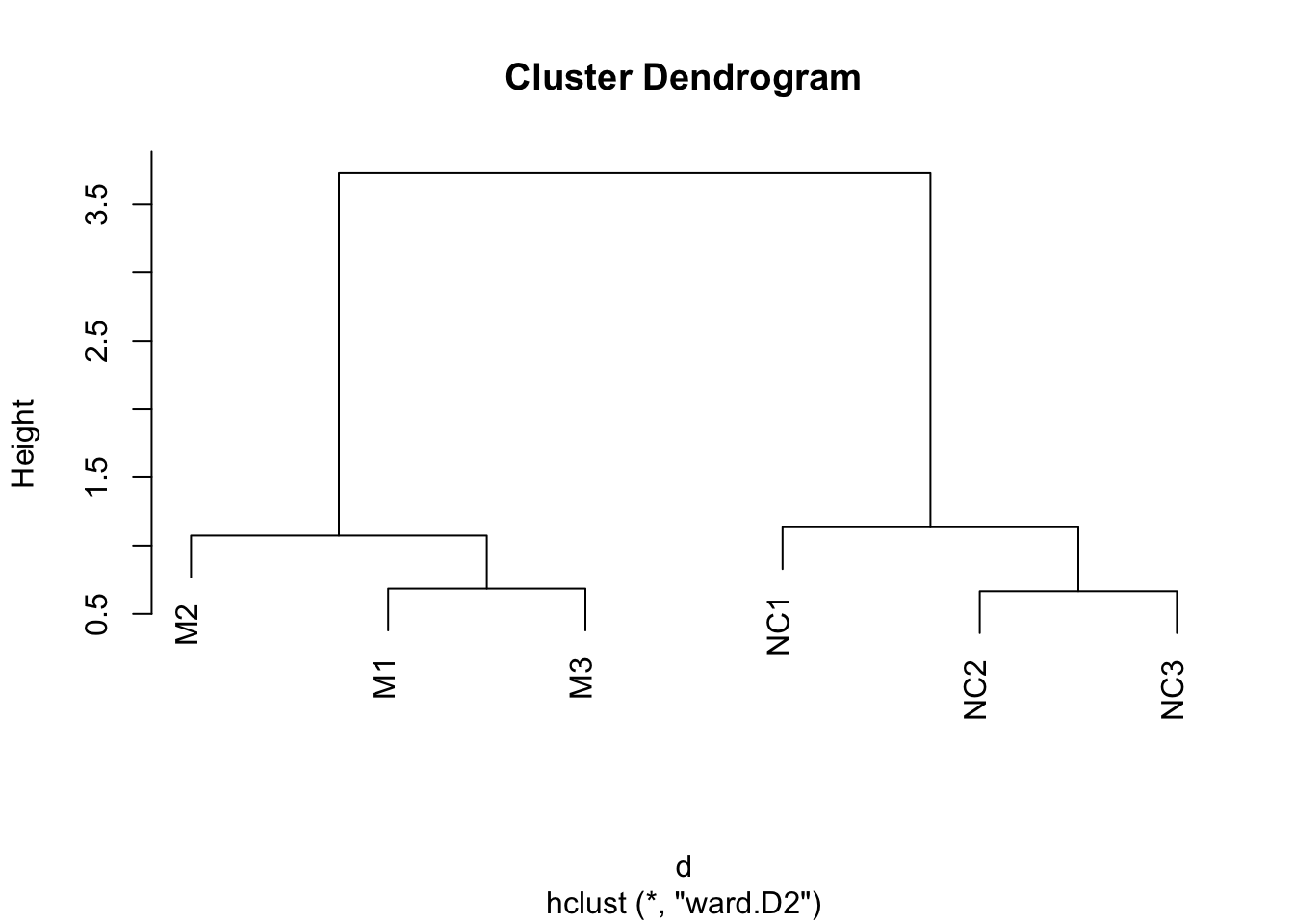
Can you guess how many clusters could best fit the data?

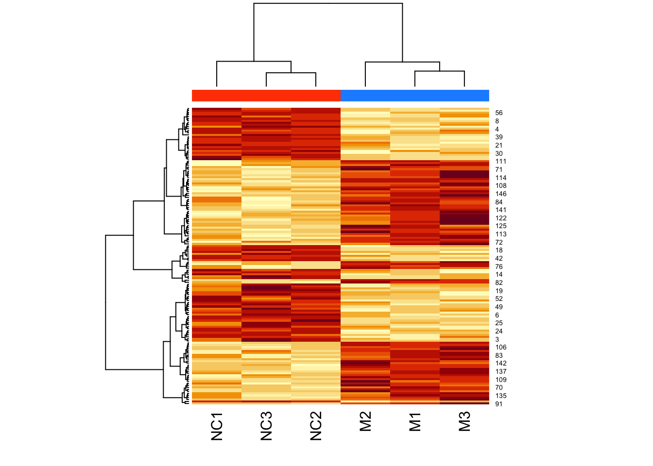
Now let’s add a heatmap to this dendrogram, so we can see the values of genes in each cluster. For this we will use the heatmap() function. First let’s just try the heatmap function:

mouse_exp <- as.matrix(mouse_exp)
heatmap(mouse_exp)

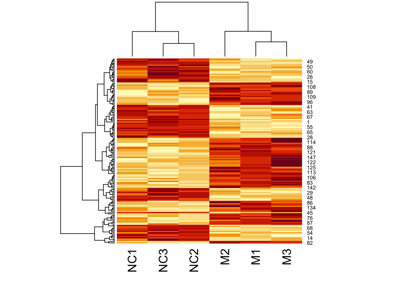
We can clearly see the data separated into two. But now let’s colour-code samples based on cluster assignments. We get cluster assignments by “cutting” the dendrogram for two clusters (something we expect from our experimental design). We use cutree() for this.

h2 <- cutree(h, k = 2)

Let’s look at our assigned labels:

h2

##  M1  M2  M3 NC1 NC2 NC3 
##   1   1   1   2   2   2

Let’s assign colours to the clusters so that cluster 1 is in pink, and cluster 2 is in green:

clust_colours <- c("pink","green")[h2]

Look at clust_colours:

clust_colours

## [1] "pink"  "pink"  "pink"  "green" "green" "green"

Now let’s plot the heatmap using these assigned cluster labels:

heatmap(mouse_exp,
    ColSideColors=clust_colours)

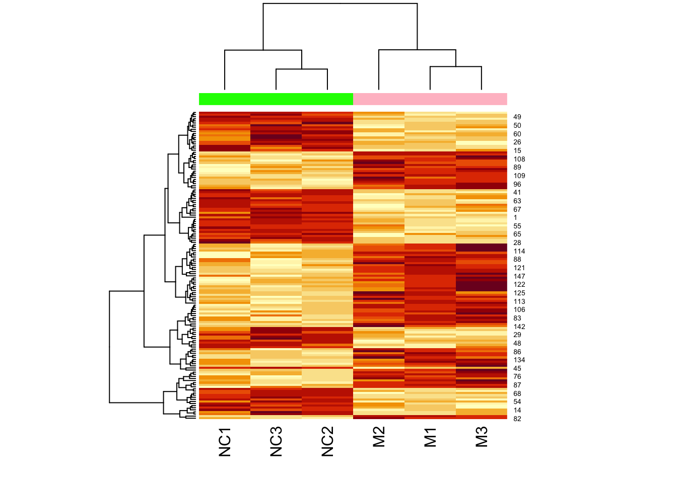
Note that the two colours are completely divided (i.e., there is no interspersed pink and green).

However, not all datasets are this simple. Let’s cluster a bladder cancer gene expression dataset. This is in the R package, bladderbatch which we have already installed.

library(bladderbatch)

## Loading required package: Biobase

## Loading required package: BiocGenerics

## Loading required package: generics

## 
## Attaching package: 'generics'

## The following objects are masked from 'package:base':
## 
##     as.difftime, as.factor, as.ordered, intersect, is.element, setdiff, setequal, union

## 
## Attaching package: 'BiocGenerics'

## The following objects are masked from 'package:stats':
## 
##     IQR, mad, sd, var, xtabs

## The following objects are masked from 'package:base':
## 
##     anyDuplicated, aperm, append, as.data.frame, basename, cbind, colnames, dirname, do.call,
##     duplicated, eval, evalq, Filter, Find, get, grep, grepl, is.unsorted, lapply, Map, mapply,
##     match, mget, order, paste, pmax, pmax.int, pmin, pmin.int, Position, rank, rbind, Reduce,
##     rownames, sapply, saveRDS, table, tapply, unique, unsplit, which.max, which.min

## Welcome to Bioconductor
## 
##     Vignettes contain introductory material; view with 'browseVignettes()'. To cite
##     Bioconductor, see 'citation("Biobase")', and for packages 'citation("pkgname")'.

Load the dataset:

data(bladderdata)

We will use specialized functions to get the expression data and sample information.

bexprs <- exprs(bladderEset)
bpheno <- pData(bladderEset)

How many genes and samples do we have in this dataset?

Let us use the same code as above to cluster these samples:

d <- dist(t(bexprs))
h <- hclust(d, method="ward.D2")
plot(h)

How many clusters do we see?

Let’s assume three clusters, and assign colours to these. As before we use cutree():

h3 <- cutree(h, k=3)
clust_colours <- c("red","green","blue")[h3]

Look at the colour assignments?

table(h3)

## h3
##  1  2  3 
## 16 27 14

Let’s just plot the heatmap.

heatmap(bexprs,
    ColSideColors=clust_colours)

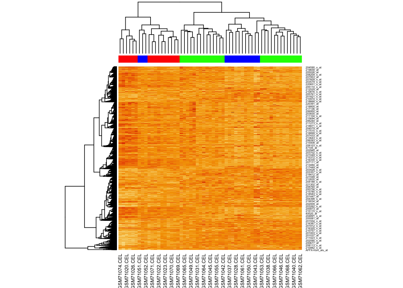
Why aren’t the samples clustering?

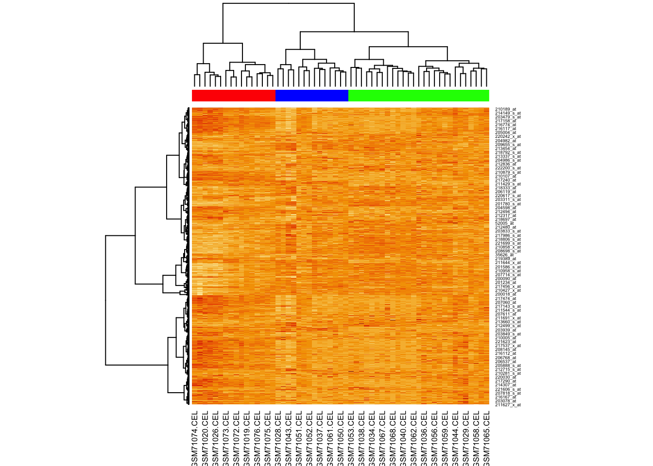
Now try providing the hclustfun to heatmap() so it uses the same method to cluster as we did. For this we will create a custom function:

myhclust <- function(x) {
    hclust(x,method="ward.D2")
}

And now we run heatmap again, using our clustering function:

heatmap(bexprs,
    ColSideColors=clust_colours,
    hclustfun=myhclust
)

K-means clustering

Let’s try using k-means clustering, asking for three clusters:

kclust <- kmeans(
    mouse_exp, 
    centers = 3
)
kclust

## K-means clustering with 3 clusters of sizes 64, 61, 22
## 
## Cluster means:
##         M1       M2       M3      NC1      NC2      NC3
## 1 5.553148 5.499583 5.642404 5.426931 5.435363 5.353342
## 2 3.947440 3.946048 4.012209 3.922949 3.950984 4.004362
## 3 7.416536 7.406216 7.414799 7.548674 7.534414 7.520608
## 
## Clustering vector:
##   1   2   3   4   5   6   7   8   9  10  11  12  13  14  15  16  17  18  19  20  21  22  23  24  25  26  27 
##   1   2   2   1   1   2   1   1   1   2   3   2   1   3   2   1   3   3   2   1   1   1   2   2   2   2   3 
##  28  29  30  31  32  33  34  35  36  37  38  39  40  41  42  43  44  45  46  47  48  49  50  51  52  53  54 
##   1   2   1   1   3   2   1   1   2   2   2   1   2   1   3   3   2   2   3   2   2   2   2   1   2   3   3 
##  55  56  57  58  59  60  61  62  63  64  65  66  67  68  69  70  71  72  73  74  75  76  77  78  79  80  81 
##   1   1   2   2   1   2   2   3   1   2   1   2   1   3   1   2   1   1   1   1   1   3   2   2   1   3   1 
##  82  83  84  85  86  87  88  89  90  91  92  93  94  95  96  97  98  99 100 101 102 103 104 105 106 107 108 
##   3   2   1   1   2   3   1   2   1   2   2   2   2   2   2   2   1   2   1   2   1   2   2   2   2   3   1 
## 109 110 111 112 113 114 115 116 117 118 119 120 121 122 123 124 125 126 127 128 129 130 131 132 133 134 135 
##   2   1   1   2   1   1   1   1   3   3   2   1   1   1   3   2   1   1   1   2   1   1   1   1   1   2   2 
## 136 137 138 139 140 141 142 143 144 145 146 147 
##   2   2   2   2   1   1   2   1   3   1   1   1 
## 
## Within cluster sum of squares by cluster:
## [1] 166.24343 193.59229  81.44264
##  (between_SS / total_SS =  74.3 %)
## 
## Available components:
## 
## [1] "cluster"      "centers"      "totss"        "withinss"     "tot.withinss" "betweenss"    "size"        
## [8] "iter"         "ifault"

Using `clValid` to determine number of clusters

Use the clValid() function to validate clusters using the:

Dunn index,
silhouette scores, and
connectivity

validation_data <- clValid(
    mouse_exp,
    2:6, # num. clusters to evaluate
    clMethods = c("hier","kmeans"), # methods to eval.
    validation = "internal"
)

Let’s look at the results:

summary(validation_data)

## 
## Clustering Methods:
##  hierarchical kmeans 
## 
## Cluster sizes:
##  2 3 4 5 6 
## 
## Validation Measures:
##                                  2       3       4       5       6
##                                                                   
## hierarchical Connectivity   5.3270 14.2528 20.7520 27.0726 30.6194
##              Dunn           0.1291  0.0788  0.0857  0.0899  0.0899
##              Silhouette     0.5133  0.4195  0.3700  0.3343  0.3233
## kmeans       Connectivity  13.2548 17.6651 37.3980 43.2655 50.6095
##              Dunn           0.0464  0.0873  0.0777  0.0815  0.0703
##              Silhouette     0.4571  0.4182  0.3615  0.3367  0.3207
## 
## Optimal Scores:
## 
##              Score  Method       Clusters
## Connectivity 5.3270 hierarchical 2       
## Dunn         0.1291 hierarchical 2       
## Silhouette   0.5133 hierarchical 2

All measures of clustering consistently indicate that two clusters best fit the data.

Now let’s cluster:

d <- dist(t(log(mouse_exp)))
h <- hclust(d,method="ward.D2")
cluster_ids <- cutree(h, k = 2)
clust_colors <- c("dodgerblue","orangered")[cluster_ids]

heatmap(
    as.matrix(mouse_exp),
    hclustfun = myhclust,
    ColSideColors = clust_colors
)

Bonus Exercise

For your exercise, try the following:

Load the MASS package using: library(MASS)
Import crabs dataset using: data(crabs)
Learn about this dataset using: ?crabs
Extract the numeric columns describing the crab measurements (“FL”, “RW”, “CL”, “CW”, “BD”)
Cluster the numeric columns using your method of choice
Plot and color your data by clusters, by species (sp), and sex
Do your clusters seem to separate these groups in the same way?