Module 5 Pan Genomics
Lab
Developed by Jimmy Liu and William Hsiao
Introduction
In this lab, we will explore how pangenome graphs can be used to model and compare sequence variations in a population of bacterial genomes. We will work with a Salmonella enterica dataset comprising a large number of cases linked to three distinct foodborne outbreaks that occurred in Quebec, Canada between 2012-2014. For a more detailed background on how the outbreaks happened, you are encouraged to review the original study by Bekal et al. (2014).
This dataset captures a wide range of sequence variations, including single-nucleotide polymorphisms (SNPs), insertions, deletions, and gene presence/absence differences among isolates. As you analyze the pangenome graph, see if you can identify these variations, describe what type of genetic changes they represent, and determine which functional elements (e.g., genes, regulatory regions, or mobile genetic elements) they occur in.
Learning Objectives
By the end of the session, you will be able to:
Describe how colored de Bruijn graphs (cDBGs) represent sequence variation across genomes.
Use Bifrost to construct and query a bacterial pangenome graph.
Visualize graph topology in Bandage and interpret structural differences.
Explain how k-mer length impacts graph complexity and biological resolution.
Part 1: Understanding the structural layout of cDBGs
Build colored de Bruijn graph (k=31)
# create a list containing paths to input genomes
find data/ -type f > refs.txt
# build cDBG
Bifrost build -r refs.txt \
              -k 31 -t 4 -c -o salmonella_k31

# Output:
#   salmonella_k31.gfa.gz     → compacted DBG in GFA format
#   salmonella_k31.colors.bfg → color information
#   salmonella_k31.bfi        → graph search index
Visualize cDBG in Bandage
To visualize the output graph (.GFA) constructed by Bifrost, you will need Bandage installed on your own computer (Not on the server!). You can find the installation guide here
For Bandage to access the output files, the files need to be transferred to your local device. All files generated on the server can be downloaded by navigating to http://##.uhn-hpc.ca/ (Replace ## with your assigned node number!)
Now open the GFA file in Bandage and click [Draw Graph]. It should take a few seconds to render the graph.
Part 2: Annotating and interpreting a pangenome graph
Alternative paths in pangenome graphs indicate sequence polymorphism, but how do we know if a polymorphism: - spans a coding sequence, intergenic region or mobile genetic element? - is found in which samples?
Analyzing a Gene or Region of Interest using BLAST
Download the spaL gene sequence from NCBI and blast the gene against all nodes of the graph to find the most likely location of the gene within the context of the pangenome graph.
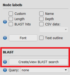
Calling BLAST in Bandage:
- Based on the graph topology, what type of mutation does the gene likely contain? Is it a SNP? Insertion? Deletion?
Next, align the unitig sequences of the nodes in the bubble structure to determine the exact genotypic difference.
Copy the exact sequence of the two nodes in the bubble structure by first selecting the two nodes -> navigating to [Output] -> [Copy selected node to clipboard].
Open BLASTN in the browser (link) and paste both sequences into the text box to align them to each other.
- How many polymorphic sites are there?
- How do the two alleles differ?
Query the pangenome graph
To determine which subset of the population contains our alleles of interest, we can use the query subcommand in Bifrost.
First save the sequences of the two alleles into a single FASTA file called query.fa, then query the FASTA file against the graph:
Bifrost query -g salmonella_k31.gfa -C salmonella_k31.colors.bfg \
              -q query.fa -o query_result.tsv -e 1.0
Output interpretation (query_result.tsv):
- Which outbreak strains share the same allele for the spaL gene?
- How do we determine every possible variation that is uniquely carried by a specific strain?
Part 3: Impact of k-mer length on graph topology
Open salmonella_k21.gfa and salmonella_k51.gfa in Bandage.
Record your observations on changes in graph topology according to this table:
| k-mer size | Graph topology |
|---|---|
| k = 21 | |
| k = 31 | |
| k = 51 |
Wrap-Up
Let’s now summarize the use the cDBG for comparative genomics and the exploration of genetic vairations across microbial pangenomes.
| Strengths | Weaknesses |
|---|---|
| Captures SNPs, indels, gene gain/loss without reference | Visualization becomes complex for many genomes |
| Unified data structure to encode pan-genome variations | Interpretation needs experience |
| Efficient querying across 1000s of genomes via colored graphs | Parameter choice (k) is critical |
| Unitigs yield greater specificity than canonical k-mers | Highly sensitive to assembly fragmentation |
Closing reflection: - How might long read sequencing impact the quality of cdBG construction?