Module 1: Data Cleaning and Exploration Review
Lab
Read in Data
Get your current working directory.
Download
Download csv file from this link: https://doi.org/10.5061/dryad.f6t39kj
Place it into your current working directory.
Read in data.
Looking at your Data
## [1] "data.frame"## [1] 6662 50## [1] "Binomial"
## [2] "Genus"
## [3] "epithet"
## [4] "valid..reptile.database..February.2018."
## [5] "year.of.description"
## [6] "country.described.from"
## [7] "main.biogeographic.Realm"
## [8] "Geographic.Range"
## [9] "known.only.from.the.only.type."
## [10] "Latitude.centroid..from.Roll.et.al..2017."
## [11] "Longitude.centroid..from.Roll.et.al..2017."
## [12] "insular.endemic"
## [13] "maximum.SVL"
## [14] "female.SVL"
## [15] "hatchling.neonate.SVL"
## [16] "Leg.development"
## [17] "mass_equation..Feldman.et.al..2016.unless.stated."
## [18] "intercept"
## [19] "slope"
## [20] "Activity.time"
## [21] "Activity.time..comments"
## [22] "substrate"
## [23] "substrate..comments"
## [24] "diet"
## [25] "diet..comments"
## [26] "foraging.mode"
## [27] "foraging.mode..comments."
## [28] "reproductive.mode"
## [29] "clutch.size"
## [30] "smallest.clutch"
## [31] "largest.clutch"
## [32] "smallest.mean.clutch.size"
## [33] "largest.mean.clutch.size"
## [34] "breeding.age..months."
## [35] "youngest.age.at.first.breeding..months."
## [36] "oldest.age.at.first.breeding..months."
## [37] "mean.body.temperature.of.active.animals.in.the.wild"
## [38] "minimum.mean.Tb"
## [39] "maximum.mean.Tb"
## [40] "Family"
## [41] "Phylogeny"
## [42] "phylogenetic.data"
## [43] "IUCN.redlist.assessment"
## [44] "IUCN.population.trend"
## [45] "Extant.Extinct"
## [46] "Remarks"
## [47] "References..Biology..all.columns.except.M..N.and.O.."
## [48] "References..SVL.of.unsexed.individuals..neonates.and.hatchlings"
## [49] "References..SVL.of.females"
## [50] "References..SVL.of.males"## [1] "Binomial"
## [2] "Genus"
## [3] "epithet"
## [4] "valid..reptile.database..February.2018."
## [5] "year.of.description"
## [6] "country.described.from"
## [7] "main.biogeographic.Realm"
## [8] "Geographic.Range"
## [9] "known.only.from.the.only.type."
## [10] "Latitude.centroid..from.Roll.et.al..2017."## Binomial Genus epithet
## 1 Ablepharus bivittatus Ablepharus bivittatus
## 2 Ablepharus budaki Ablepharus budaki
## 3 Ablepharus chernovi Ablepharus chernovi
## 4 Ablepharus darvazi Ablepharus darvazi
## 5 Ablepharus deserti Ablepharus deserti
## 6 Ablepharus grayanus Ablepharus grayanus
## 7 Ablepharus kitaibelii Ablepharus kitaibelii
## 8 Ablepharus lindbergi Ablepharus lindbergi
## 9 Ablepharus pannonicus Ablepharus pannonicus
## 10 Ablepharus rueppellii Ablepharus rueppellii
## valid..reptile.database..February.2018. year.of.description
## 1 yes 1832
## 2 yes 1996
## 3 yes 1953
## 4 yes 1990
## 5 yes 1868
## 6 yes 1872
## 7 yes 1833
## 8 yes 1960
## 9 yes 1824
## 10 yes 1839
## country.described.from main.biogeographic.Realm
## 1 Azerbaijan Palearctic
## 2 Turkey Palearctic
## 3 Armenia Palearctic
## 4 Tajikistan Palearctic
## 5 Uzbekistan Palearctic
## 6 India Oriental
## 7 Greece Palearctic
## 8 Afghanistan Palearctic
## 9 Uzbekistan Palearctic
## 10 Jordan Palearctic
## Geographic.Range
## 1 Armenia, Azerbaijan, Turkmenistan, Iran, Turkey
## 2 Cyprus, Lebanon, Syria, Turkey
## 3 Armenia, Turkey
## 4 Tajikistan
## 5 Kazakhstan to Tadjikistan
## 6 India, Pakistan, Iran
## 7 Greece (Aegean islands: Paros, Antiparos, Despotiko, Strongylo, Tourlos, Preza, Glaropunta, Panteronisi, Cyprus, Rhodos, Peloponnes, Syphnos, Corfu, Lesbos, Samos, Samothraki, Milos, Tinos), Romania, Bulgaria, Yugoslavia, Hungary, Albania, Czechoslovakia, Russia, Turkey, Syria, Iraq ?, Egypt (Sinai), Lebanon?
## 8 Afghanistan
## 9 Georgia, Turkmenistan, Tajikistan, Uzbekistan, Kyrgyzstan, Azerbaijan, Iran, Iraq, Oman, Afghanistan, Pakistan, Jordan?, Syria, United Arab Emirates (UAE), India
## 10 Egypt, Israel, Jordan, Lebanon, Syria,
## known.only.from.the.only.type. Latitude.centroid..from.Roll.et.al..2017.
## 1 no 34.16
## 2 no 36.44
## 3 no 38.32
## 4 no 38.96
## 5 no 41.38
## 6 no 27.09
## 7 no 41.11
## 8 no 34.28
## 9 no 33.16
## 10 no 31.39
## Longitude.centroid..from.Roll.et.al..2017. insular.endemic maximum.SVL
## 1 53.20 no 61
## 2 34.06 no 48
## 3 37.95 no 54
## 4 69.79 no 44
## 5 68.40 no 58.8
## 6 70.93 no 34.9
## 7 25.77 no 58
## 8 66.28 no 50
## 9 58.67 no 55
## 10 35.28 no 52
## female.SVL hatchling.neonate.SVL Leg.development
## 1 56.5 18.5 four-legged
## 2 36.8 <NA> four-legged
## 3 44.4 <NA> four-legged
## 4 <NA> <NA> four-legged
## 5 46 17.5 four-legged
## 6 <NA> 14.5 four-legged
## 7 43.4 20 four-legged
## 8 <NA> <NA> four-legged
## 9 <NA> 20 four-legged
## 10 35.3 18.5 four-legged
## mass_equation..Feldman.et.al..2016.unless.stated. intercept slope
## 1 Legged Scincidae -5.125 3.229
## 2 Legged Scincidae -5.125 3.229
## 3 Legged Scincidae -5.125 3.229
## 4 Legged Scincidae -5.125 3.229
## 5 Legged Scincidae -5.125 3.229
## 6 Legged Scincidae -5.125 3.229
## 7 Legged Scincidae -5.125 3.229
## 8 Legged Scincidae -5.125 3.229
## 9 Legged Scincidae -5.125 3.229
## 10 Legged Scincidae -5.125 3.229
## Activity.time
## 1 Diurnal
## 2 Diurnal
## 3 Diurnal
## 4 Diurnal
## 5 Diurnal
## 6 Diurnal
## 7 Diurnal
## 8 Diurnal
## 9 Diurnal
## 10 Diurnal
## Activity.time..comments
## 1 Diurnal
## 2 Diurnal
## 3 Diurnal
## 4 Diurnal (Philipp Wagner Personal communication to Enav Vidan, October 2015)
## 5 Diurnal (Jablonski 2016 and inferred from Szczerbak 2003)
## 6 Diurnal (e.g., Karamiani et al. 2018)
## 7 Diurnal (e.g., pers. obs., Speybroeck et al. 2016, Stille and Stille 2017)/ crepuscular (Valakos et al. 2008)
## 8 Diurnal (Nasrullah Rastegar-Pouyani Personal communication to Enav Vidan, October 2015)
## 9 Diurnal (e.g., Karamiani et al. 2018)
## 10 Diurnal (e.g., pers obs. And Werner 2016)
## substrate substrate..comments
## 1 Saxicolous Saxicolous
## 2 Terrestrial Leaf litter
## 3 Saxicolous Saxicolous
## 4 <NA> <NA>
## 5 Terrestrial Terrestrial (Szczerbak, Jablonski 2016)
## 6 Terrestrial Terrestrial and Leaf Litter (e.g., Greer 1973)
## 7 Terrestrial Leaf Litter (e.g., pers. pbs. And Vergilov and Natchev 2017)
## 8 <NA> <NA>
## 9 Terrestrial Leaf Litter
## 10 Terrestrial Leaf Litter (e.g., pers. obs. And Werner 2016)
## diet
## 1 Carnivorous
## 2 Carnivorous
## 3 Carnivorous
## 4 <NA>
## 5 Carnivorous
## 6 Carnivorous
## 7 Carnivorous
## 8 <NA>
## 9 Carnivorous
## 10 Carnivorous
## diet..comments
## 1 Invertebrates ("Food consists mainly of insects (beetles, hymenopterans, and cicadas), spiders, and snails", Szczerbak 2003)
## 2 Invertebrates
## 3 Arthropods ("ants, flies, aphids, small beetles, and spiders.", Szczerbak 2003)
## 4 <NA>
## 5 Arthropods ("beetles, caterpillars, and cicadas) and spiders" Szczerbak 2003)
## 6 Insects (Mostly ants)
## 7 Invertebrates (spiders and earthworms, Street 1979, Rogner 1997b), small invertebrates (Stille and Stille 2017)
## 8 <NA>
## 9 Arthropods (beetles and spiders, Szczerbak 2003)
## 10 arthropods (Amitai and Bouskila 2001)
## foraging.mode foraging.mode..comments. reproductive.mode
## 1 <NA> <NA> Oviparous
## 2 <NA> <NA> Oviparous
## 3 <NA> <NA> Oviparous
## 4 <NA> <NA> <NA>
## 5 <NA> <NA> Oviparous
## 6 <NA> <NA> Oviparous
## 7 <NA> <NA> Oviparous
## 8 <NA> <NA> <NA>
## 9 <NA> <NA> Oviparous
## 10 <NA> <NA> Oviparous
## clutch.size
## 1 3-5, usually 4 (Arakelyan et al. 2011), 4-5 (Szczerbak 2003)
## 2 <NA>
## 3 3 (n=1, Szczerbak 2003)
## 4 <NA>
## 5 1-8 (Szczerbak 2003)
## 6 <NA>
## 7 2-4 (Stojanov et al. 2011, Speybroeck et al. 2016, Kwet 2015), up to 4 (Stille and Stille 2017), max 5 (Vergilov et al. 2018)
## 8 4.5 (Myhrvold et al. 2015)
## 9 2-3 (Ataev et al. 1994), 3-4 (Gardner 2013), 3-6 (Szczerbak 2003)
## 10 up to 3 (Bar and Haimovitch 2012), 1-2, mean 1.5 (Goldberg 2013, TAU experimental zoo data), mean 2.1 (Werner 1995), 1-3, mean 2.1 (Werner 2016)
## smallest.clutch largest.clutch smallest.mean.clutch.size
## 1 2 5 4.0
## 2 2 5 NA
## 3 3 4 NA
## 4 NA NA NA
## 5 1 8 NA
## 6 1 2 NA
## 7 2 6 NA
## 8 4 5 4.5
## 9 2 6 NA
## 10 1 6 1.5
## largest.mean.clutch.size
## 1 4.0
## 2 NA
## 3 NA
## 4 NA
## 5 NA
## 6 NA
## 7 NA
## 8 4.5
## 9 NA
## 10 2.1
## breeding.age..months.
## 1 <NA>
## 2 <NA>
## 3 <NA>
## 4 <NA>
## 5 Szczerbak 2003: 10 months
## 6 <NA>
## 7 6 month for 35mm which is min adult size, fig 2 (Vergilov et al. 2018)
## 8 <NA>
## 9 Ataev et al. 1994: 10-11 months, Szczerbak 2003: 1 year
## 10 <NA>
## youngest.age.at.first.breeding..months.
## 1 NA
## 2 NA
## 3 NA
## 4 NA
## 5 10
## 6 NA
## 7 6
## 8 NA
## 9 10
## 10 NA
## oldest.age.at.first.breeding..months.
## 1 NA
## 2 NA
## 3 NA
## 4 NA
## 5 10
## 6 NA
## 7 6
## 8 NA
## 9 12
## 10 NA
## mean.body.temperature.of.active.animals.in.the.wild
## 1 <NA>
## 2 <NA>
## 3 <NA>
## 4 <NA>
## 5 <NA>
## 6 <NA>
## 7 Shai pers. obs. (n=1, 27 deg)
## 8 <NA>
## 9 <NA>
## 10 Roll et al. 2013 (25.6-34.8) but it should be 29.5, for n=5 active animals (Meiri, pers. Obs. 15.4.2014)
## minimum.mean.Tb maximum.mean.Tb Family
## 1 NA NA Scincidae
## 2 NA NA Scincidae
## 3 NA NA Scincidae
## 4 NA NA Scincidae
## 5 NA NA Scincidae
## 6 NA NA Scincidae
## 7 27.0 27.0 Scincidae
## 8 NA NA Scincidae
## 9 NA NA Scincidae
## 10 29.5 29.5 Scincidae
## Phylogeny
## 1 <NA>
## 2 Pyron and Burbrink 2014, Skourtanioti et al. 2016
## 3 Pyron and Burbrink 2014, Skourtanioti et al. 2016
## 4 <NA>
## 5 <NA>
## 6 <NA>
## 7 Pyron and Burbrink 2014, Skourtanioti et al. 2016
## 8 <NA>
## 9 Pyron and Burbrink 2014, Skourtanioti et al. 2016
## 10 Skourtanioti et al. 2016
## phylogenetic.data IUCN.redlist.assessment
## 1 <NA> LC
## 2 2mt and 2 nuclear genes (Skourtanioti et al. 2016) LC
## 3 2mt and 2 nuclear genes (Skourtanioti et al. 2016) LC
## 4 <NA> DD
## 5 <NA> LC
## 6 <NA> NE
## 7 2mt and 2 nuclear genes (Skourtanioti et al. 2016) LC
## 8 <NA> LC
## 9 2mt and 2 nuclear genes (Skourtanioti et al. 2016) NE
## 10 2mt and 2 nuclear genes (Skourtanioti et al. 2016) LC
## IUCN.population.trend Extant.Extinct
## 1 decreasing extant
## 2 stable extant
## 3 stable extant
## 4 unknown extant
## 5 unknown extant
## 6 NE extant
## 7 stable extant
## 8 unknown extant
## 9 NE extant
## 10 unknown extant
## Remarks
## 1 <NA>
## 2 <NA>
## 3 <NA>
## 4 <NA>
## 5 <NA>
## 6 <NA>
## 7 <NA>
## 8 <NA>
## 9 <NA>
## 10 elevational data (0-1660): Meiri, own data
## References..Biology..all.columns.except.M..N.and.O..
## 1 Szczerbak 2003, Anderson 1999, Baran and Atatur 1998, Clark 1990, Arakelyan et al. 2011
## 2 Gocmen et al. 1996, Baier et al. 2009, Schmidtler 1997, Franzen et al. 2008
## 3 Szczerbak 2003, Baran and Atatur 1998, Schmidtler 1997, Arakelyan et al. 2011
## 4 <NA>
## 5 Szczerbak 2003, Jablonski 2016
## 6 Minton 1966, Tikader and Sharma 1992, Greene 1982, Khan 2006, Greer 1973, Karamiani et al. 2018
## 7 Arnold and Ovenden 2004, Baran and Atatur 1998, Street 1979, Rogner 1997b, Atatur and Gocmen 2001, Herczeg et al. 2007, Valakos et al. 2008, Valakos et al. 2004, Arbel 1984, Kwet 2009, Kohler 2005, Schmidtler 1997, Stojanov et al. 2011, Tomovic et al. 2015, Speybroeck et al. 2016, Kwet 2015, Vergilov et al. 2016, Vergilov and Natchev 2017, Stille and Stille 2017, Vergilov et al. 2018
## 8 <NA>
## 9 Smith 1935, Szczerbak 2003, Anderson 1999, Arnold 1972, Khan 2006, Clark 1990, Jongbloed 2000, Eremchenko 2007, Weber 1960, van der Kooij 2001, Fathinia et al. 2009, Grossmann et al. 2012, Ataev et al. 1994, Gardner 2013, Karamiani et al. 2018
## 10 Amitai and Bouskila 2001, Arbel 1984, Disi et al. 2001, El Din 2006, Bar and Haimovitch 2012, Roll et al. 2013, Goldberg 2013, Werner 1995, Werner 2016, TAU experimental zoo data
## References..SVL.of.unsexed.individuals..neonates.and.hatchlings
## 1 Szczerbak 2003, Boulenger 1887, Arakelyan et al. 2011,
## 2 Gocmen et al. 1996, Franzen et al. 2008,
## 3 Szczerbak 2003, Arakelyan et al. 2011,
## 4 <NA>
## 5 Szczerbak 2003, Boulenger 1887,
## 6 Smith 1935, Minton 1966, Tikader and Sharma 1992, Boulenger 1890, Boulenger 1887, Khan 2006, Karamiani et al. 2015, Ali et al. 2017,
## 7 Arnold and Ovenden 2004,Herczeg et al. 2007, Foufopoulos and Ives 1999, Franzen et al. 2008, Stojanov et al. 2011, Vergilov et al. 2018
## 8 Wettstein 1960,
## 9 Smith 1935, Szczerbak 2003, Anderson 1999, Minton 1966, Boulenger 1890, Boulenger 1887, Khan 2006, Jongbloed 2000, Arnold 1986, Werner 1930, Gardner 2013, Karamiani et al. 2015,
## 10 Meiri (own measurements), Maza 2008, TAU Herpetology collection, El Din 2006, Roll et al. 2013,
## References..SVL.of.females
## 1 Anderson 1999, Ahmadzadeh et al. 2008, Arakelyan et al. 2011,
## 2 Gocmen et al. 1996, Budak et al. 1998, Baier et al. 2009, Schmidtler 1997,
## 3 Schmidtler 1997,
## 4 <NA>
## 5 Jablonski 2016,
## 6 <NA>
## 7 Fitch 1981, Arnold and Ovenden 2004, Disi et al. 2001, El Din 2006, Schmidtler 1997, Stojanov et al. 2011, Vergilov et al. 2018
## 8 <NA>
## 9 <NA>
## 10 Disi et al. 2001, Schmidtler 1997, Goldberg 2012, TAUM collection, Werner 1995, Werner 2016,
## References..SVL.of.males
## 1 Anderson 1999,
## 2 Gocmen et al. 1996, Budak et al. 1998, Baier et al. 2009, Schmidtler 1997,
## 3 Schmidtler 1997,
## 4 Yeriomchenko and Panfilov 1990,
## 5 <NA>
## 6 <NA>
## 7 Fitch 1981, Arnold and Ovenden 2004, Disi et al. 2001, Schmidtler 1997, Stojanov et al. 2011, Vergilov et al. 2018
## 8 <NA>
## 9 Fathinia et al. 2009,
## 10 Disi et al. 2001, Schmidtler 1997, Goldberg 2012,# We have a lot of columns. Let's subset to remove columns we don't need for now.
dfTraits <- dfReptiles %>% ## tidyverse pipe
# Select function allows us to choose the columns we want
select(c(Binomial, Genus, Family,
main.biogeographic.Realm, Latitude.centroid..from.Roll.et.al..2017.,
insular.endemic, maximum.SVL, hatchling.neonate.SVL, Leg.development,
Activity.time, substrate, diet, foraging.mode, reproductive.mode,
smallest.clutch, largest.clutch, youngest.age.at.first.breeding..months.,
IUCN.redlist.assessment, IUCN.population.trend, Extant.Extinct
))
names(dfTraits)## [1] "Binomial"
## [2] "Genus"
## [3] "Family"
## [4] "main.biogeographic.Realm"
## [5] "Latitude.centroid..from.Roll.et.al..2017."
## [6] "insular.endemic"
## [7] "maximum.SVL"
## [8] "hatchling.neonate.SVL"
## [9] "Leg.development"
## [10] "Activity.time"
## [11] "substrate"
## [12] "diet"
## [13] "foraging.mode"
## [14] "reproductive.mode"
## [15] "smallest.clutch"
## [16] "largest.clutch"
## [17] "youngest.age.at.first.breeding..months."
## [18] "IUCN.redlist.assessment"
## [19] "IUCN.population.trend"
## [20] "Extant.Extinct"# Let's clean up these column names!
names(dfTraits) <- tolower(names(dfTraits))
# Replace all "." with "_" (personal preference)
names(dfTraits) <- gsub("\\.", "_", names(dfTraits))
names(dfTraits)## [1] "binomial"
## [2] "genus"
## [3] "family"
## [4] "main_biogeographic_realm"
## [5] "latitude_centroid__from_roll_et_al__2017_"
## [6] "insular_endemic"
## [7] "maximum_svl"
## [8] "hatchling_neonate_svl"
## [9] "leg_development"
## [10] "activity_time"
## [11] "substrate"
## [12] "diet"
## [13] "foraging_mode"
## [14] "reproductive_mode"
## [15] "smallest_clutch"
## [16] "largest_clutch"
## [17] "youngest_age_at_first_breeding__months_"
## [18] "iucn_redlist_assessment"
## [19] "iucn_population_trend"
## [20] "extant_extinct"# Make some of the names shorter.
names(dfTraits)[5] <- "latitude"
names(dfTraits)[17] <- "age_first_breeding"
names(dfTraits)[17]## [1] "age_first_breeding"# Rename species column.
names(dfTraits)[1] <- "species"
# In order to properly count the number of missing values, replace blanks with NAs
# I always do this just in case.
dfTraits[dfTraits == " "] <- NA# Make sure there are no species name duplications.
# Note that using the sum() function on logical vector will count the number of TRUE values.
duplicated(dfTraits$species)
sum(duplicated(dfTraits$species))# Are there any species that don't have ANY data?
missRows <- apply(dfTraits[, -(1:3)], MARGIN = 1, function(x) all(is.na(x)))
# Let's break that down! First, we ed if "x" row had NAs.
is.na(dfTraits[1, ]) ## logical vector## species genus family main_biogeographic_realm latitude insular_endemic
## 1 FALSE FALSE FALSE FALSE FALSE FALSE
## maximum_svl hatchling_neonate_svl leg_development activity_time substrate
## 1 FALSE FALSE FALSE FALSE FALSE
## diet foraging_mode reproductive_mode smallest_clutch largest_clutch
## 1 FALSE TRUE FALSE FALSE FALSE
## age_first_breeding iucn_redlist_assessment iucn_population_trend
## 1 TRUE FALSE FALSE
## extant_extinct
## 1 FALSE## species genus family main_biogeographic_realm latitude
## 1 Ablepharus bivittatus Ablepharus Scincidae Palearctic 34.16
## insular_endemic maximum_svl hatchling_neonate_svl leg_development
## 1 no 61 18.5 four-legged
## activity_time substrate diet foraging_mode reproductive_mode
## 1 Diurnal Saxicolous Carnivorous <NA> Oviparous
## smallest_clutch largest_clutch age_first_breeding iucn_redlist_assessment
## 1 2 5 NA LC
## iucn_population_trend extant_extinct
## 1 decreasing extant## [1] TRUE# Note you could use the "any" function to if ANY of the elements are NA
any() ## There are a couple NAs## [1] FALSE# Then we "apply" that function to all of the rows (MARGIN = 1) in the dataframe which returns:
missRows## [1] 0Working with Different Data Types
Let’s try to understand the type of data we are working with.
##  [1] "species"                  "genus"
##  [3] "family"                   "main_biogeographic_realm"
##  [5] "latitude"                 "insular_endemic"
##  [7] "maximum_svl"              "hatchling_neonate_svl"
##  [9] "leg_development"          "activity_time"
## [11] "substrate"                "diet"
## [13] "foraging_mode"            "reproductive_mode"
## [15] "smallest_clutch"          "largest_clutch"
## [17] "age_first_breeding"       "iucn_redlist_assessment"
## [19] "iucn_population_trend"    "extant_extinct"
# First, let's ID which columns are taxonomic information so we don't include them in our summary stats.
taxCols <- c("species", "genus", "family")
# The rest are traits
traits <- setdiff(names(dfTraits), taxCols)
traits## [1] "main_biogeographic_realm" "latitude"
## [3] "insular_endemic" "maximum_svl"
## [5] "hatchling_neonate_svl" "leg_development"
## [7] "activity_time" "substrate"
## [9] "diet" "foraging_mode"
## [11] "reproductive_mode" "smallest_clutch"
## [13] "largest_clutch" "age_first_breeding"
## [15] "iucn_redlist_assessment" "iucn_population_trend"
## [17] "extant_extinct"## main_biogeographic_realm latitude insular_endemic
## "character" "numeric" "character"
## maximum_svl hatchling_neonate_svl leg_development
## "character" "character" "character"
## activity_time substrate diet
## "character" "character" "character"
## foraging_mode reproductive_mode smallest_clutch
## "character" "character" "integer"
## largest_clutch age_first_breeding iucn_redlist_assessment
## "integer" "numeric" "character"
## iucn_population_trend extant_extinct
## "character" "character"# Let's ID which traits are numerical and which are categorical.
index <- sapply(dfTraits[traits], is.numeric)
index## main_biogeographic_realm latitude insular_endemic
## FALSE TRUE FALSE
## maximum_svl hatchling_neonate_svl leg_development
## FALSE FALSE FALSE
## activity_time substrate diet
## FALSE FALSE FALSE
## foraging_mode reproductive_mode smallest_clutch
## FALSE FALSE TRUE
## largest_clutch age_first_breeding iucn_redlist_assessment
## TRUE TRUE FALSE
## iucn_population_trend extant_extinct
## FALSE FALSE## [1] "character"## species genus family main_biogeographic_realm latitude
## 1 Ablepharus bivittatus Ablepharus Scincidae Palearctic 34.16
## 2 Ablepharus budaki Ablepharus Scincidae Palearctic 36.44
## 3 Ablepharus chernovi Ablepharus Scincidae Palearctic 38.32
## 4 Ablepharus darvazi Ablepharus Scincidae Palearctic 38.96
## 5 Ablepharus deserti Ablepharus Scincidae Palearctic 41.38
## 6 Ablepharus grayanus Ablepharus Scincidae Oriental 27.09
## insular_endemic maximum_svl hatchling_neonate_svl leg_development
## 1 no 61 18.5 four-legged
## 2 no 48 <NA> four-legged
## 3 no 54 <NA> four-legged
## 4 no 44 <NA> four-legged
## 5 no 58.8 17.5 four-legged
## 6 no 34.9 14.5 four-legged
## activity_time substrate diet foraging_mode reproductive_mode
## 1 Diurnal Saxicolous Carnivorous <NA> Oviparous
## 2 Diurnal Terrestrial Carnivorous <NA> Oviparous
## 3 Diurnal Saxicolous Carnivorous <NA> Oviparous
## 4 Diurnal <NA> <NA> <NA> <NA>
## 5 Diurnal Terrestrial Carnivorous <NA> Oviparous
## 6 Diurnal Terrestrial Carnivorous <NA> Oviparous
## smallest_clutch largest_clutch age_first_breeding iucn_redlist_assessment
## 1 2 5 NA LC
## 2 2 5 NA LC
## 3 3 4 NA LC
## 4 NA NA NA DD
## 5 1 8 10 LC
## 6 1 2 NA NE
## iucn_population_trend extant_extinct
## 1 decreasing extant
## 2 stable extant
## 3 stable extant
## 4 unknown extant
## 5 unknown extant
## 6 NE extant# The column has strings mixed with numbers, which returns a character vector.
# We should replace the strings with NAs.
# Here, we are using regex to match any letter and then replacing the matches with NAs.
dfTraits$maximum_svl <- gsub(pattern = "[a-zA-Z]", replacement = NA, x = dfTraits$maximum_svl)
dfTraits$hatchling_neonate_svl <- gsub("[a-zA-Z]", NA, dfTraits$hatchling_neonate_svl)
# Change both traits to numeric.
# Note here I am using lapply to apply the function for the columns of dfTraits.
# Note: lapply returns a list, sapply returns a vector. "map" would be the tidyverse equivalent of apply, lapply, sapply, etc. functions.
dfTraits[, c("maximum_svl", "hatchling_neonate_svl")] <- lapply(dfTraits[, c("maximum_svl", "hatchling_neonate_svl")], as.numeric)
class(dfTraits$maximum_svl)## [1] "numeric"# Let's try IDing our numerical traits again.
index <- sapply(dfTraits[traits], is.numeric)
# Subset the column names using indexing.
contTraits <- traits[index]
contTraits ## is this right?## [1] "latitude" "maximum_svl" "hatchling_neonate_svl"
## [4] "smallest_clutch" "largest_clutch" "age_first_breeding"# Get the categorical traits.
catTraits <- setdiff(traits, contTraits)
# Convert character to factor because this is helpful for summary stats and plotting.
# It is also the data class that regression models require for categorical variables.
dfTraits[catTraits] <- lapply(dfTraits[catTraits], as.factor)
# If you wanted to make a particular category within a variable the reference.
# Important for statistical analyses with categorical variables.
table(dfTraits$insular_endemic)##
## no unknown yes
## 5 4612 1 2044dfTraits$insular_endemic <- relevel(dfTraits$insular_endemic, "no")
# One last .
sapply(dfTraits, class)## species genus family
## "character" "character" "character"
## main_biogeographic_realm latitude insular_endemic
## "factor" "numeric" "factor"
## maximum_svl hatchling_neonate_svl leg_development
## "numeric" "numeric" "factor"
## activity_time substrate diet
## "factor" "factor" "factor"
## foraging_mode reproductive_mode smallest_clutch
## "factor" "factor" "integer"
## largest_clutch age_first_breeding iucn_redlist_assessment
## "integer" "numeric" "factor"
## iucn_population_trend extant_extinct
## "factor" "factor"Summary Stats
Some base R summary statistics to get a quick look at your data.
##    species             genus              family
##  Length:6662        Length:6662        Length:6662
##  Class :character   Class :character   Class :character
##  Mode  :character   Mode  :character   Mode  :character
##
##
##
##
##  main_biogeographic_realm    latitude         insular_endemic  maximum_svl
##  Neotropic :2041          Min.   :-50.65000   no     :4612    Min.   :  17.0
##  Oriental  :1167          1st Qu.:-17.89500          :   5    1st Qu.:  56.0
##  Afrotropic:1009          Median :  1.66000   unknown:   1    Median :  75.9
##  Australia : 772          Mean   :  0.03201   yes    :2044    Mean   :  95.7
##  Palearctic: 555          3rd Qu.: 17.21500                   3rd Qu.: 105.0
##  (Other)   :1117          Max.   : 56.60000                   Max.   :1570.0
##  NA's      :   1          NA's   :31                          NA's   :29
##  hatchling_neonate_svl       leg_development    activity_time
##  Min.   :  8.10                      :   5             :   5
##  1st Qu.: 23.00        forelimbs only:  10   Cathemeral: 268
##  Median : 28.00        four-legged   :5992   Diurnal   :3578
##  Mean   : 33.62        hindlimbs only:  64   Nocturnal :1247
##  3rd Qu.: 36.00        leg-reduced   : 188   NA's      :1564
##  Max.   :174.50        Limbless      : 403
##  NA's   :4589
##                 substrate             diet              foraging_mode
##  Terrestrial         :1750              :   5                  :   5
##  Arboreal            :1083   Carnivorous:2685   active foraging: 514
##  Saxicolous          : 848   Herbivorous: 159   mixed          :  96
##  Arboreal&Terrestrial: 486   Omnivorous : 515   Sit and Wait   : 460
##  Arboreal&Saxicolous : 295   NA's       :3298   NA's           :5587
##  (Other)             :1187
##  NA's                :1013
##   reproductive_mode smallest_clutch  largest_clutch   age_first_breeding
##            :   5    Min.   : 1.000   Min.   : 1.000   Min.   :  1.00
##  Mixed     :  20    1st Qu.: 1.000   1st Qu.: 2.000   1st Qu.:  9.00
##  Oviparous :3309    Median : 2.000   Median : 3.000   Median : 12.00
##  unclear   :  11    Mean   : 2.534   Mean   : 5.675   Mean   : 18.53
##  Viviparous: 714    3rd Qu.: 3.000   3rd Qu.: 7.000   3rd Qu.: 24.00
##  NA's      :2603    Max.   :34.000   Max.   :95.000   Max.   :144.00
##                     NA's   :3067     NA's   :3067     NA's   :5961
##  iucn_redlist_assessment iucn_population_trend extant_extinct
##  NE     :3021                      :   5              :   5
##  LC     :2148            decreasing: 565       EW     :   2
##  DD     : 453            increasing:  18       extant :6612
##  EN     : 322            NE        :3097       extinct:  43
##  VU     : 278            stable    :1372
##  NT     : 253            unknown   :1605
##  (Other): 187
Time for some tidyverse magic!
Use of the tidyverse pipe avoids us having to create several interim variables while also improving readability.
# Say we only wanted to keep extant species:
dfTraits <- dfTraits %>%
  # Filter function allows us to apply a condition to our data.
  filter(extant_extinct == "extant") %>%
  # Remove column using minus sign as we no longer need it
  select(-extant_extinct)

# Remove trait from catTraits.
catTraits
## [1] "main_biogeographic_realm" "insular_endemic"
## [3] "leg_development" "activity_time"
## [5] "substrate" "diet"
## [7] "foraging_mode" "reproductive_mode"
## [9] "iucn_redlist_assessment" "iucn_population_trend"
## [11] "extant_extinct"catTraits <- catTraits[-11]
# Other summary info.
# How many families do we have?
unique(dfTraits$family)## [1] "Scincidae" "Anguidae" "Agamidae"
## [4] "Lacertidae" "Gymnophthalmidae" "Eublepharidae"
## [7] "Gekkonidae" "Trogonophiidae" "Diplodactylidae"
## [10] "Iguanidae" "Teiidae" "Amphisbaenidae"
## [13] "Dibamidae" "Leiosauridae" "Anniellidae"
## [16] "Dactyloidae" "Pygopodidae" "Chamaeleonidae"
## [19] "Sphaerodactylidae" "Phyllodactylidae" "Corytophanidae"
## [22] "Bipedidae" "Blanidae" "Gerrhosauridae"
## [25] "Cadeidae" "Phrynosomatidae" "Carphodactylidae"
## [28] "Opluridae" "Cordylidae" "Xantusiidae"
## [31] "Crotaphytidae" "Liolaemidae" "Hoplocercidae"
## [34] "Tropiduridae" "Helodermatidae" "Lanthanotidae"
## [37] "Leiocephalidae" "Polychrotidae" "Rhineuridae"
## [40] "Shinisauridae" "Varanidae" "Xenosauridae"## [1] 42# Top 10 Families with most species.
# You can sort by increasing or decreasing number of species.
head(sort(table(dfTraits$family), decreasing = T), n = 10)##
## Scincidae Gekkonidae Agamidae Dactyloidae
## 1622 1159 487 426
## Lacertidae Liolaemidae Gymnophthalmidae Sphaerodactylidae
## 328 308 265 216
## Chamaeleonidae Amphisbaenidae
## 207 175# Doing the same thing, but with tidyverse syntax
dfTraits %>%
dplyr::count(family, sort = T) %>% ## to make sure the count function isn't masked
head(n = 10)## family n
## 1 Scincidae 1622
## 2 Gekkonidae 1159
## 3 Agamidae 487
## 4 Dactyloidae 426
## 5 Lacertidae 328
## 6 Liolaemidae 308
## 7 Gymnophthalmidae 265
## 8 Sphaerodactylidae 216
## 9 Chamaeleonidae 207
## 10 Amphisbaenidae 175# Sample size (number of complete observations for this trait)
head(na.omit(dfTraits$maximum_svl)) ## na.omit removes NAs from the vector## [1] 61.0 48.0 54.0 44.0 58.8 34.9## [1] 6588# Mean of the data
mean(dfTraits$maximum_svl, na.rm = T) ## has option for removing number of NAs in the function## [1] 95.35199## [1] 17 1570## [1] 24## [1] 0.003629764# To speed things up, (l)apply these to all of the numerical traits using an anonymous function.
# An anonymous function is a function without a name that you really only need temporarily
# e.g., within the confines of this lapply call.
l_contInfo <- lapply(dfTraits[contTraits], function(x){
# Number of complete observations
n <- length(na.omit(x))
# Mean
avg <- mean(x, na.rm = T)
# Number of NAs
numNAs <- sum(is.na(x))
# Proportion of NAs
propNAs <- sum(is.na(x)) / length(x)
# Return in dataframe format
return(data.frame(n, avg, numNAs, propNAs))
})
# View the first element of the list.
head(l_contInfo[[1]])## n avg numNAs propNAs
## 1 6587 -0.005732503 25 0.003781004# Bind list of dataframes together by using the do.call() function.
# This lets you rbind() the entire list of dataframes.
dfContInfo <- do.call(rbind, l_contInfo)
head(dfContInfo)## n avg numNAs propNAs
## latitude 6587 -0.005732503 25 0.003781004
## maximum_svl 6588 95.351988464 24 0.003629764
## hatchling_neonate_svl 2072 33.623262548 4540 0.686630369
## smallest_clutch 3582 2.528475712 3030 0.458257713
## largest_clutch 3582 5.681183696 3030 0.458257713
## age_first_breeding 699 18.466666667 5913 0.894283122## $main_biogeographic_realm
##
## Afrotropic Australia Madagascar Nearctic Neotropic Oceania
## 0 1004 772 332 226 2011 548
## Oriental Palearctic
## 1164 554
##
## $insular_endemic
##
## no unknown yes
## 4610 0 1 2001
##
## $leg_development
##
## forelimbs only four-legged hindlimbs only leg-reduced
## 0 10 5949 63 187
## Limbless
## 403
##
## $activity_time
##
## Cathemeral Diurnal Nocturnal
## 0 267 3570 1243
##
## $substrate
##
## Arboreal
## 0 1080
## Arboreal&Saxicolous Arboreal&Saxicolous&Terrestrial
## 294 203
## Arboreal&Terrestrial Cryptic
## 486 62
## Cryptic&Fossorial Cryptic&Terrestrial
## 12 7
## Fossorial Fossorial&Saxicolous
## 254 1
## Fossorial&Saxicolous&Terrestrial Fossorial&Terrestrial
## 6 270
## marine Saxicolous
## 1 847
## Saxicolous&Terrestrial Saxisolous
## 243 1
## Semi_Aquatic Terrestrial
## 121 1742
##
## $diet
##
## Carnivorous Herbivorous Omnivorous
## 0 2681 157 509
##
## $foraging_mode
##
## active foraging mixed Sit and Wait
## 0 512 96 460
##
## $reproductive_mode
##
## Mixed Oviparous unclear Viviparous
## 0 20 3304 11 707
##
## $iucn_redlist_assessment
##
## CR DD EN EW EX LC LR/lc LR/nt NE NT VU
## 0 139 451 322 0 0 2148 4 8 3009 253 278
##
## $iucn_population_trend
##
## decreasing increasing NE stable unknown
## 0 561 18 3070 1371 1592l_catInfo <- lapply(dfTraits[catTraits], function(x){
n <- length(na.omit(x))
# number of unique categories instead of mean for example
cats <- length(unique(x))
numNAs <- sum(is.na(x))
propNAs <- sum(is.na(x)) / length(x)
return(data.frame(n, cats, numNAs, propNAs))
})
# Bind together list.
dfCatInfo <- do.call(rbind, l_catInfo)
head(dfCatInfo)## n cats numNAs propNAs
## main_biogeographic_realm 6611 9 1 0.0001512402
## insular_endemic 6612 3 0 0.0000000000
## leg_development 6612 5 0 0.0000000000
## activity_time 5080 4 1532 0.2316999395
## substrate 5630 18 982 0.1485178463
## diet 3347 4 3265 0.4937991531# Tidyverse has handy functions for getting summary data by group.
# For example, if we wanted to get summary information grouped by family:
summary_stats1 <- dfTraits %>%
# Group by family
group_by(family) %>%
# Get the mean max SVL for each group and put it into a new column called avg_length
summarize(avg_length = mean(maximum_svl, na.rm = T)) %>%
# Arrange in descending order
arrange(desc(avg_length)) %>%
# Print to console
print()## # A tibble: 42 × 2
## family avg_length
## <chr> <dbl>
## 1 Varanidae 472.
## 2 Helodermatidae 441
## 3 Rhineuridae 380
## 4 Iguanidae 364.
## 5 Cadeidae 270
## 6 Amphisbaenidae 267.
## 7 Bipedidae 223
## 8 Blanidae 220.
## 9 Lanthanotidae 220
## 10 Corytophanidae 184.
## # ℹ 32 more rows# Let's add some info on other traits
summary_stats2 <- dfTraits %>%
group_by(family) %>%
summarize(
avg_length = mean(maximum_svl, na.rm = T),
# Average largest clutch
avg_lc = mean(largest_clutch, na.rm = T),
# Most common diet in each family
top_diet = names(sort(table(diet), decreasing = T)[1]),
) %>%
print()## # A tibble: 42 × 4
## family avg_length avg_lc top_diet
## <chr> <dbl> <dbl> <chr>
## 1 Agamidae 110. 8.98 Carnivorous
## 2 Amphisbaenidae 267. 4.22 Carnivorous
## 3 Anguidae 151. 12.2 Carnivorous
## 4 Anniellidae 156. 2.33 Carnivorous
## 5 Bipedidae 223 4 Carnivorous
## 6 Blanidae 220. 2 Carnivorous
## 7 Cadeidae 270 2 Carnivorous
## 8 Carphodactylidae 109. 2.04 Carnivorous
## 9 Chamaeleonidae 94.8 19.5 Carnivorous
## 10 Cordylidae 104. 4.08 Carnivorous
## # ℹ 32 more rowsExploratory Plots
Let’s perform some data visualization to identify patterns and variable associations in our dataset.
# Base R histograms for numerical traits
hist(dfTraits$maximum_svl) ## there are some VERY long species!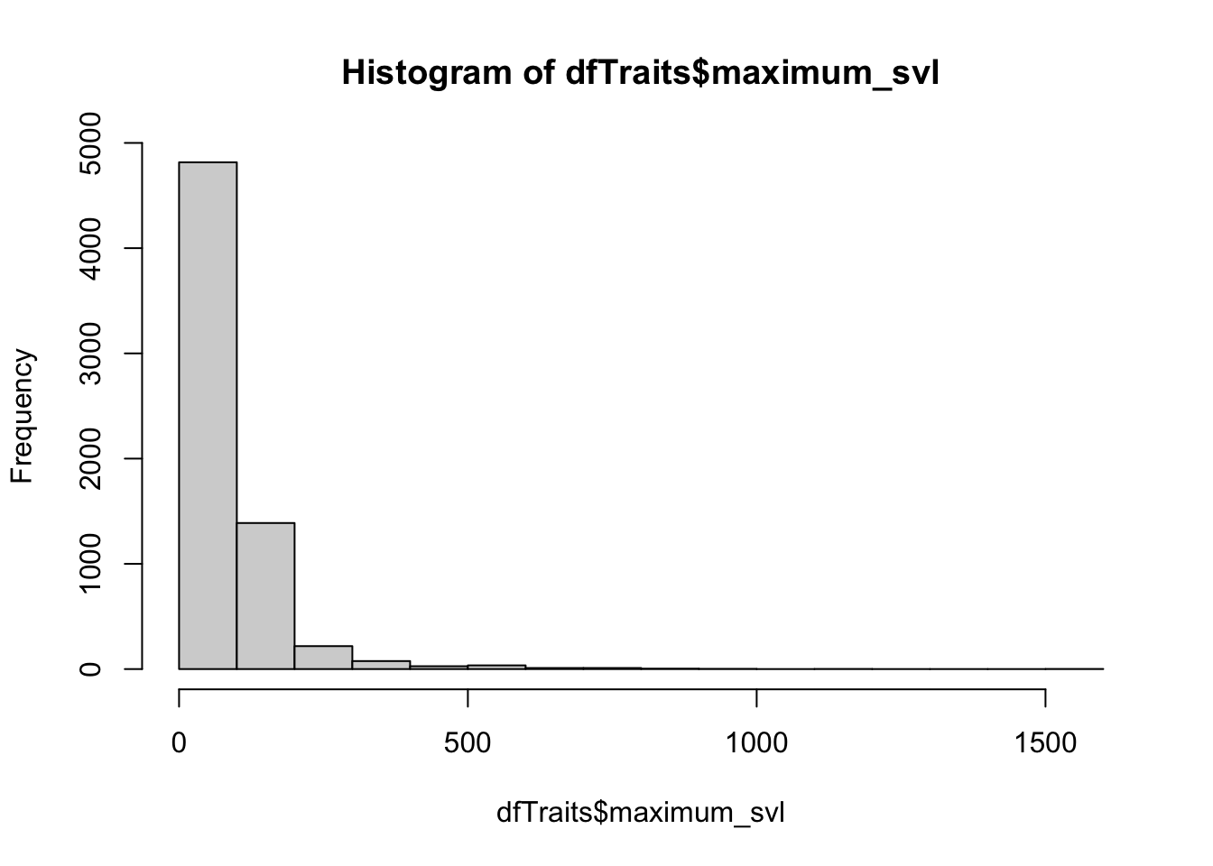
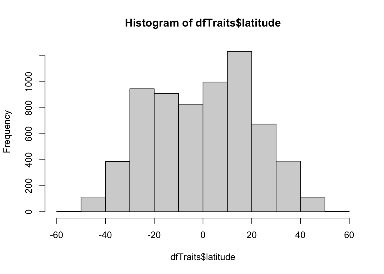
# ggplot to beautify the data
# ggplot is a very powerful tool for visualizing data but you need to get used to the syntax
ggplot(dfTraits) + ## note use of "+" over "%>%
  # Plot a histogram and make it blue.
  # geom_* indicates what type of plot you want. aes = aesthetic mapping
  geom_histogram(mapping = aes(x = latitude),
                 fill = "skyblue", colour = "black") +
  # Add labels
  labs(title = "Reptile Latitude",
       x = "Latitude (°)", y = "Count") +
  # Change the plot theme (here, making the background white)
  theme_minimal(base_size = 12) +
  # Change the theme and make some font adjustments
  theme(plot.title = element_text(hjust = 0.5, face = "bold"))
## `stat_bin()` using `bins = 30`. Pick better value with
## `binwidth`.## Warning: Removed 25 rows containing non-finite outside the scale range
## (`stat_bin()`).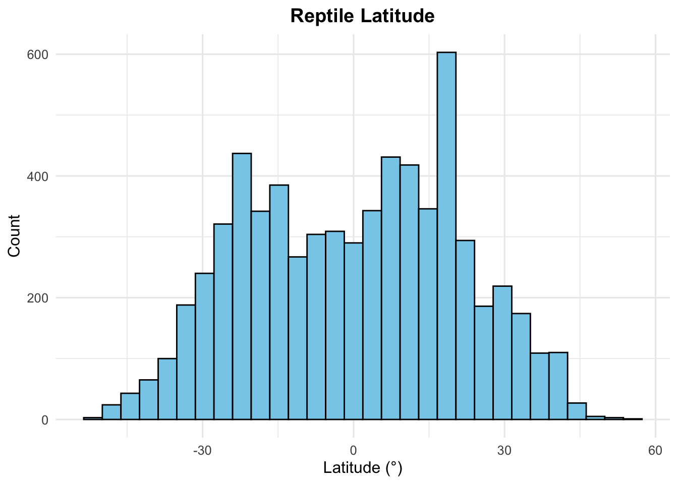
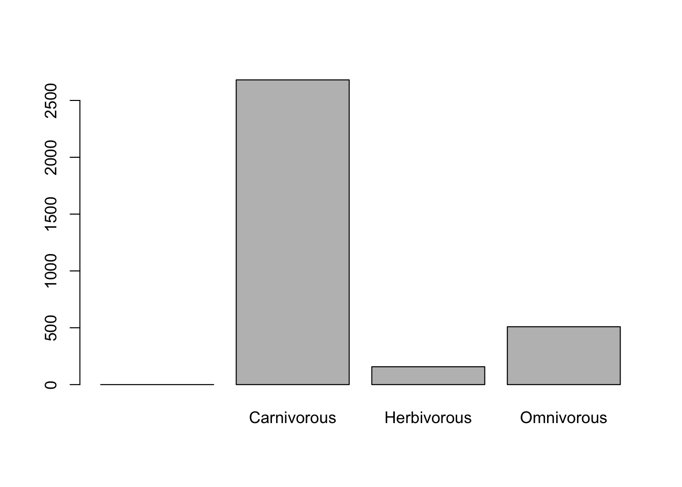
# ggplot version
# Get rid of those pesky NAs for plotting
ggplot(data = dfTraits %>% filter(!is.na(diet))) +
  # Barplot
  geom_bar(mapping = aes(x = diet, fill = diet), width = 0.7) +
  # Custom colours
  scale_fill_brewer(palette = "Paired") +
  labs(title = "Diet Types in Reptiles",
       x = "Diet",
       y = "Count") +
  theme_minimal(base_size = 12) +
  theme(plot.title = element_text(hjust = 0.5, face = "bold"),
        legend.position = "none")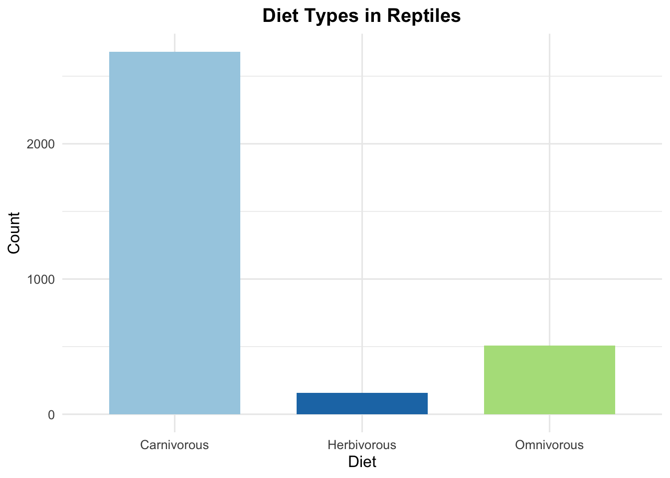
?scale_fill_brewer ## Lots of options, including colour blind friendly options

# Relationships between numerical variables
plot(dfTraits[contTraits]) ## scatter plots for each pair of traits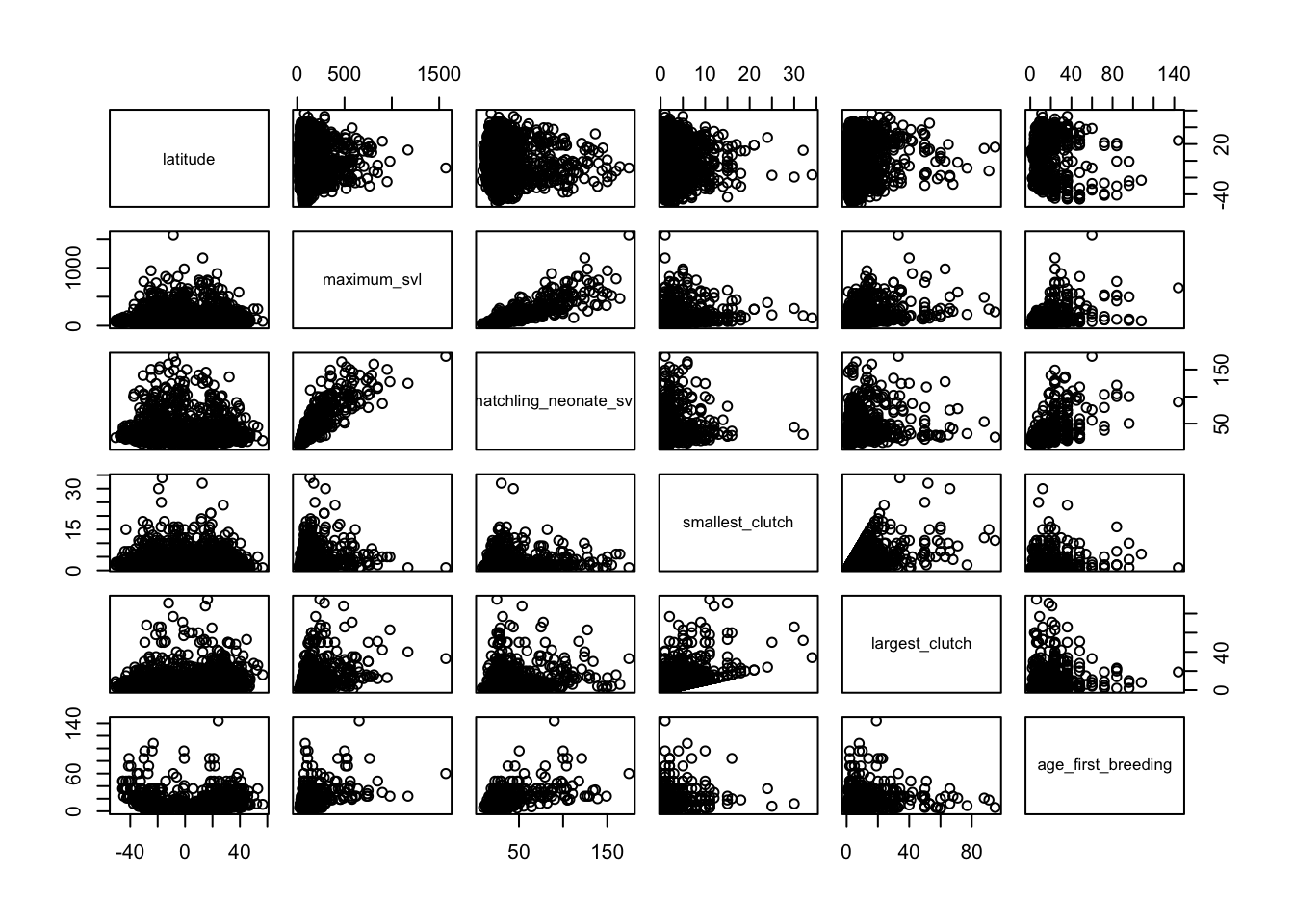
# Correlations
# Ranges from -1 to 1 and gives insight about the strength of pairwise relationships
?cor
# Note that you have the option to use different coefficients (Pearson, Kendall, Spearman)
cor(dfTraits[contTraits], use = "pairwise.complete.obs")
## latitude maximum_svl hatchling_neonate_svl
## latitude 1.000000000 -0.008342921 -0.08613691
## maximum_svl -0.008342921 1.000000000 0.85991210
## hatchling_neonate_svl -0.086136910 0.859912101 1.00000000
## smallest_clutch -0.003149907 0.243497717 0.16379773
## largest_clutch 0.094788426 0.472278560 0.27042185
## age_first_breeding -0.111217181 0.406792723 0.52252633
## smallest_clutch largest_clutch age_first_breeding
## latitude -0.003149907 0.09478843 -0.11121718
## maximum_svl 0.243497717 0.47227856 0.40679272
## hatchling_neonate_svl 0.163797729 0.27042185 0.52252633
## smallest_clutch 1.000000000 0.55075538 0.10747271
## largest_clutch 0.550755384 1.00000000 0.06566284
## age_first_breeding 0.107472714 0.06566284 1.00000000# Test for significant association between two traits
cor.test(dfTraits$hatchling_neonate_svl, dfTraits$age_first_breeding)##
## Pearson's product-moment correlation
##
## data: dfTraits$hatchling_neonate_svl and dfTraits$age_first_breeding
## t = 14.785, df = 582, p-value < 2.2e-16
## alternative hypothesis: true correlation is not equal to 0
## 95 percent confidence interval:
## 0.4609332 0.5791094
## sample estimates:
## cor
## 0.5225263# The output tells us there is a statistically significant correlation (p-value < 0.05) between these two variables.
# Quick ggplot to see relationship
ggplot(data = dfTraits) +
geom_point(mapping = aes(x = age_first_breeding, y = hatchling_neonate_svl))## Warning: Removed 6028 rows containing missing values or values outside the
## scale range (`geom_point()`).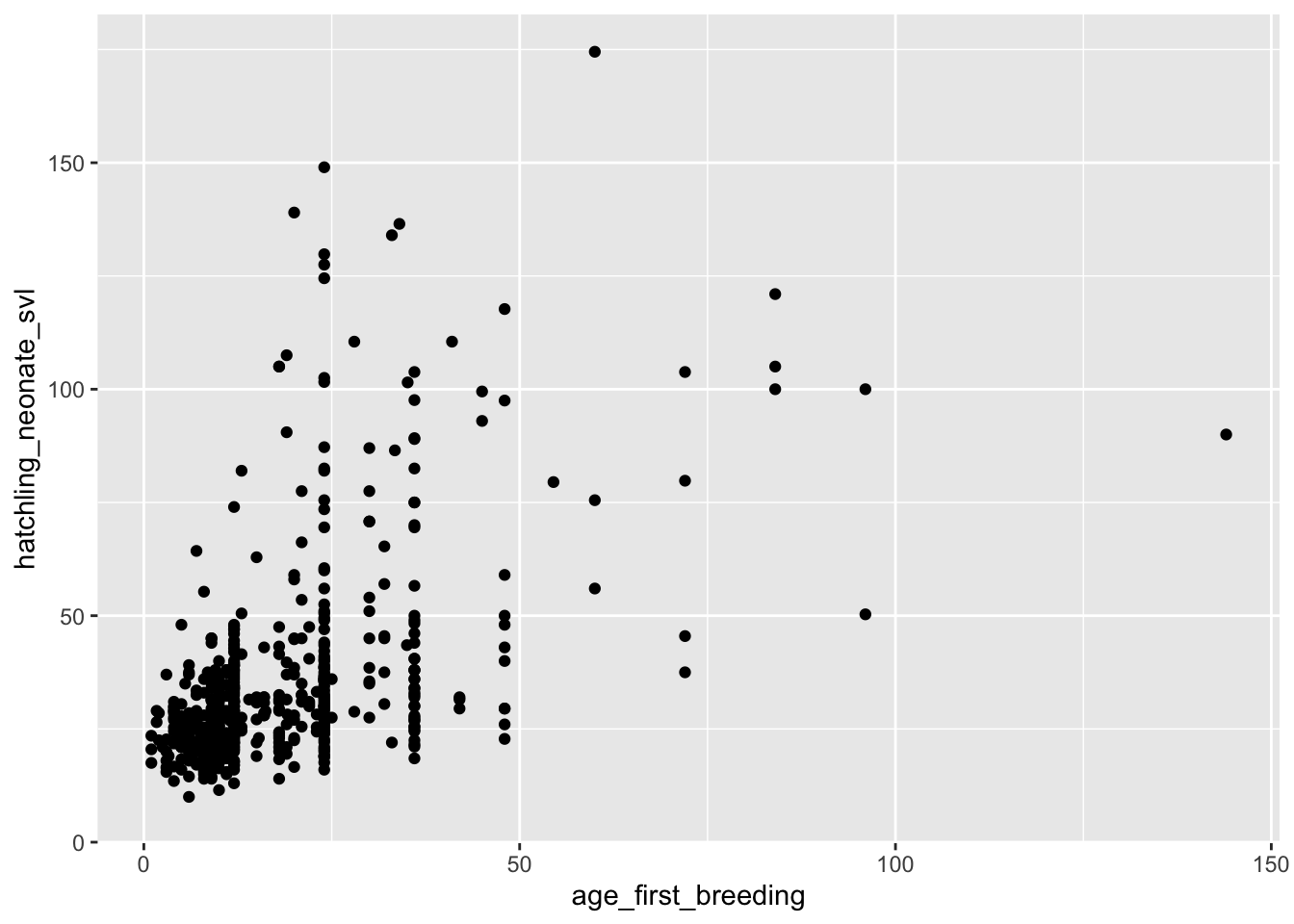
# Are these data normally distributed? We can  this using QQ plots.
hist(dfTraits$hatchling_neonate_svl)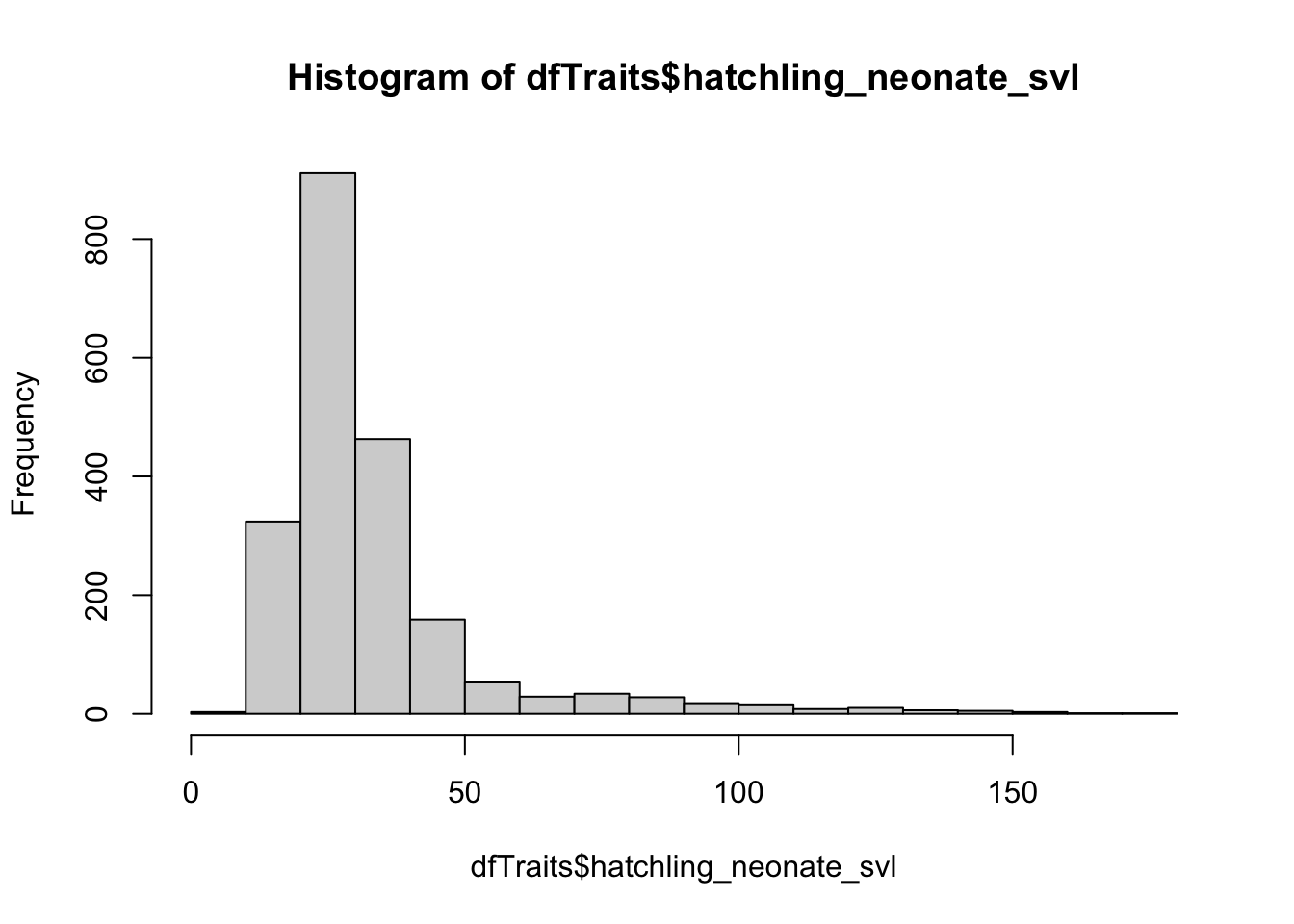
# The x-axis is the quantiles from the theoretical distribution we are comparing to (i.e., normal distribution) and y-axis is the quantiles from our data
qqnorm(dfTraits$hatchling_neonate_svl)
qqline(dfTraits$hatchling_neonate_svl) ## skewed distribution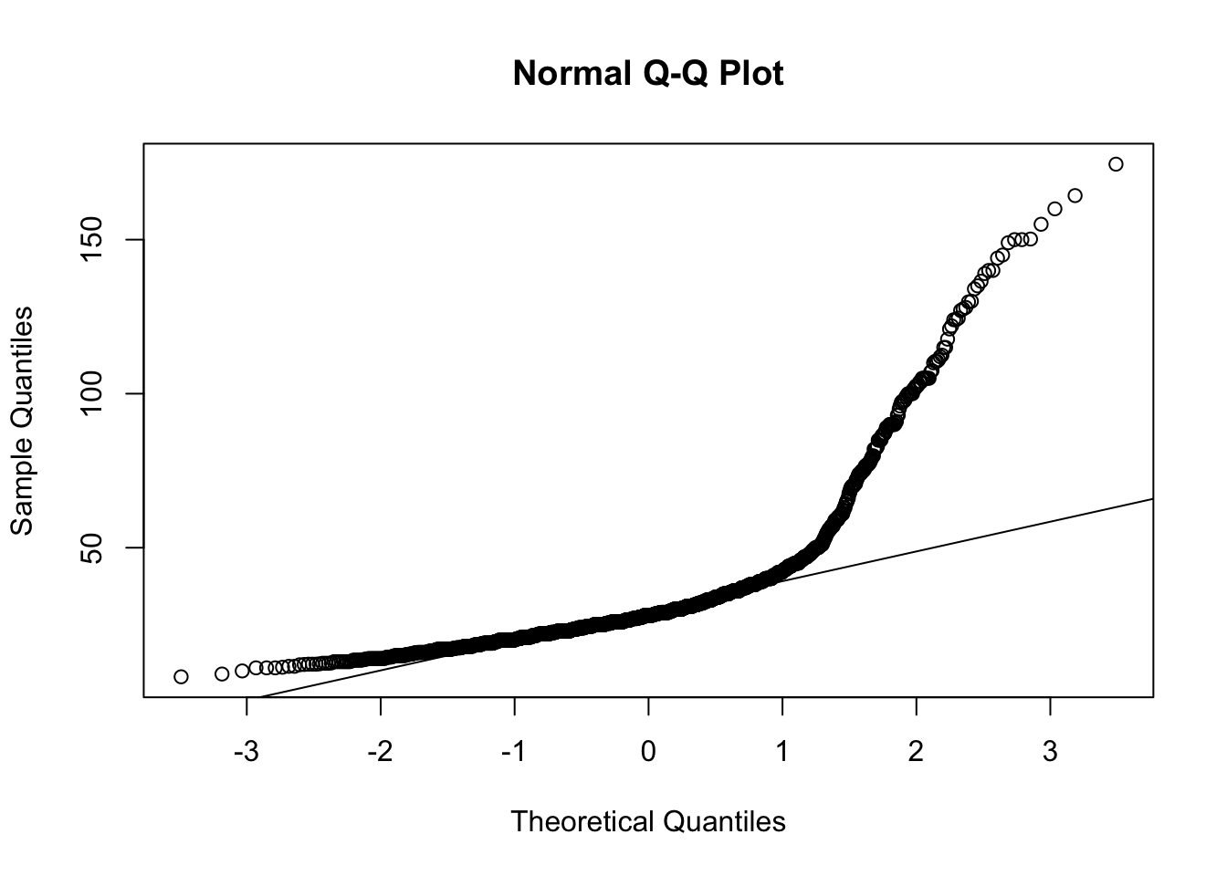
# Let' see if we can use a log-transformation to make our data resemble a normal distribution
hist(dfTraits$hatchling_neonate_svl)
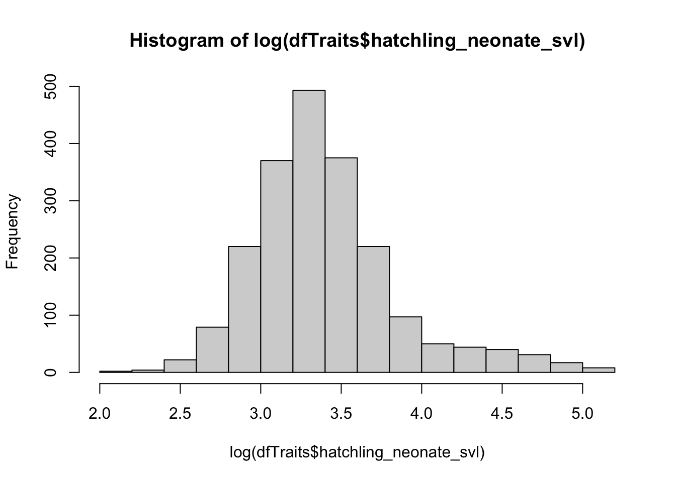
qqnorm(log(dfTraits$hatchling_neonate_svl))
qqline(log(dfTraits$hatchling_neonate_svl)) ## it helps!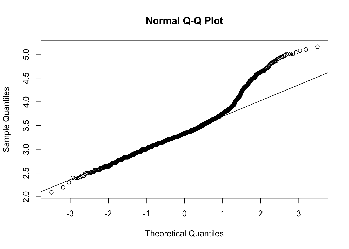
# If you wanted to keep the original data in your dataset, you could use the mutate function to create a new column with the log-transformed data
dfTraits <- dfTraits %>%
  mutate(log_hatchling_neonate_svl = log(hatchling_neonate_svl),
         log_age_first_breeding = log(age_first_breeding))
names(dfTraits)
## [1] "species" "genus"
## [3] "family" "main_biogeographic_realm"
## [5] "latitude" "insular_endemic"
## [7] "maximum_svl" "hatchling_neonate_svl"
## [9] "leg_development" "activity_time"
## [11] "substrate" "diet"
## [13] "foraging_mode" "reproductive_mode"
## [15] "smallest_clutch" "largest_clutch"
## [17] "age_first_breeding" "iucn_redlist_assessment"
## [19] "iucn_population_trend" "log_hatchling_neonate_svl"
## [21] "log_age_first_breeding"# Plot the transformed data.
# Note I placed the x and y variables in the ggplot argument here so I don't have to do it twice for both geom_point and geom_smooth
ggplot(data = dfTraits, aes(x = log_hatchling_neonate_svl, y = log_age_first_breeding)) +
geom_point(# Adding some colour and transparency (alpha) to the points
color = "skyblue", size = 2, alpha = 0.7) +
# Add linear regression line
geom_smooth(method = "lm", color = "darkblue", linewidth = 0.5) +
theme_minimal(base_size = 12)## `geom_smooth()` using formula = 'y ~ x'## Warning: Removed 6028 rows containing non-finite outside the scale range
## (`stat_smooth()`).## Warning: Removed 6028 rows containing missing values or values outside the
## scale range (`geom_point()`).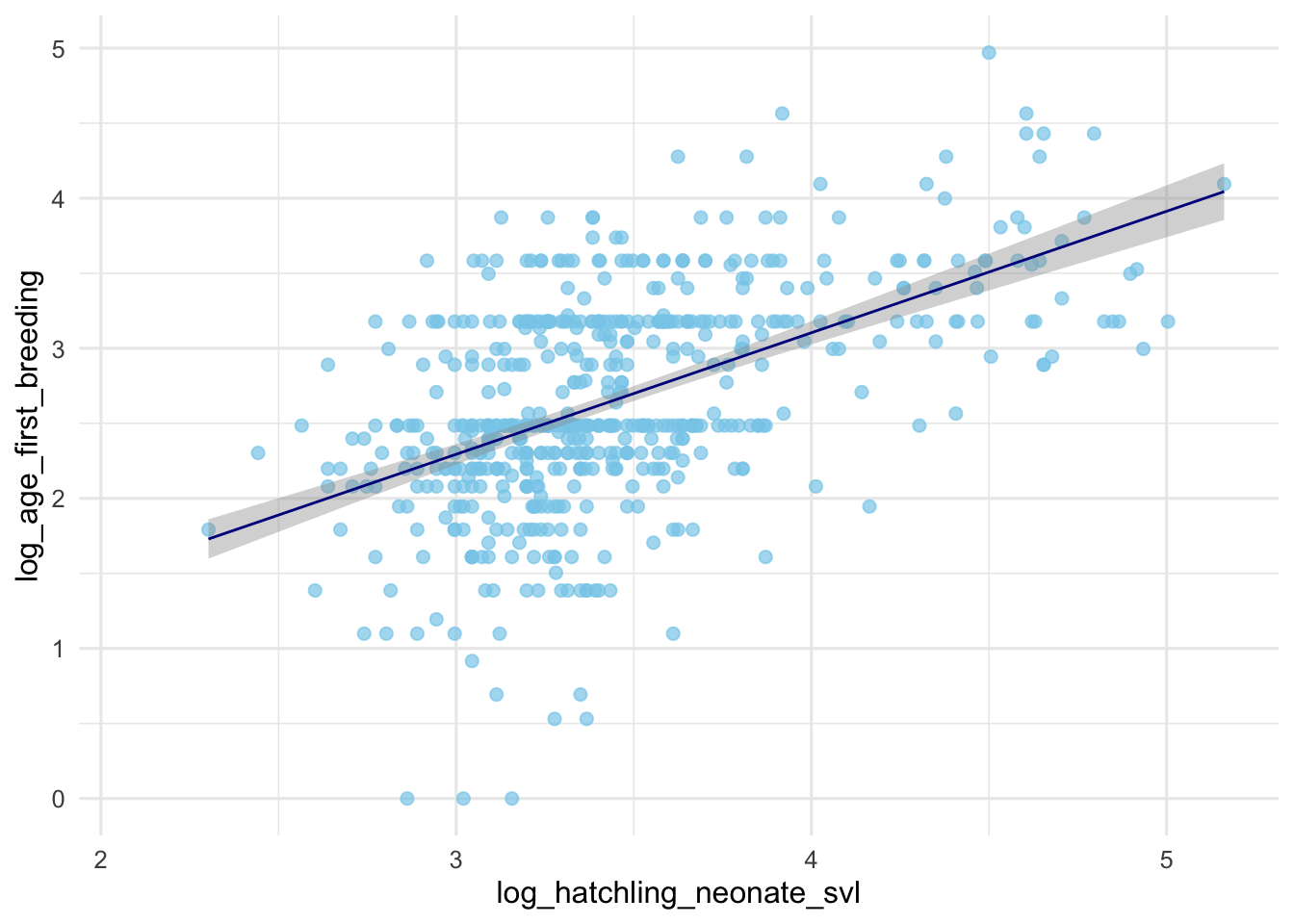
# Boxplots to show distributions of SVL by IUCN redlist assessment
ggplot(data = dfTraits, mapping = aes(x = iucn_redlist_assessment, y = log(maximum_svl))) +
# Boxplot
geom_boxplot(aes(fill = iucn_redlist_assessment)) +
scale_fill_brewer(palette = "Blues") +
labs(title = "SVL Distribution by IUCN Redlist Assessment in Reptiles",
x = "IUCN Redlist Assessment",
y = "Log Maximum SVL") +
# Flipping the coordinates for better visualization
coord_flip() +
theme_minimal(base_size = 12) +
theme(legend.position = "none") ## remove the legend## Warning: Removed 24 rows containing non-finite outside the scale range
## (`stat_boxplot()`).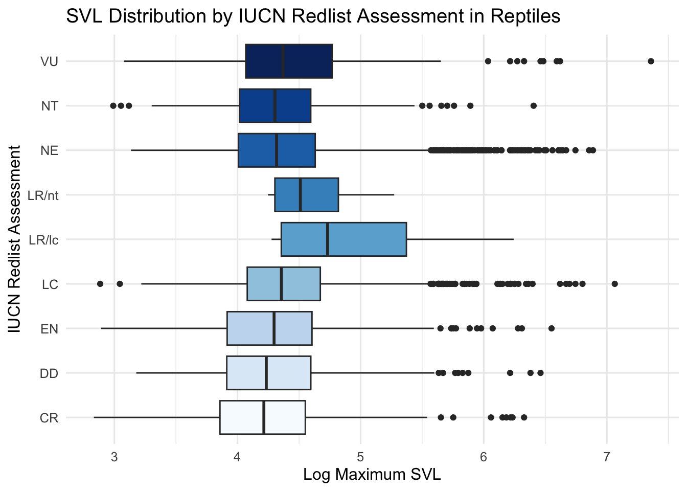
# Associations between categorical variables.
ggplot(data = dfTraits %>% filter(!is.na(diet))) +
# Using a variant of geom_point
geom_count(mapping = aes(x = diet, y = iucn_redlist_assessment)) +
labs(x = "Diet",
y = "IUCN Redlist Assessment") +
# Increasing the size of the points
scale_size_continuous(range = c(2, 10), name = "Count") +
theme_minimal(base_size = 12) 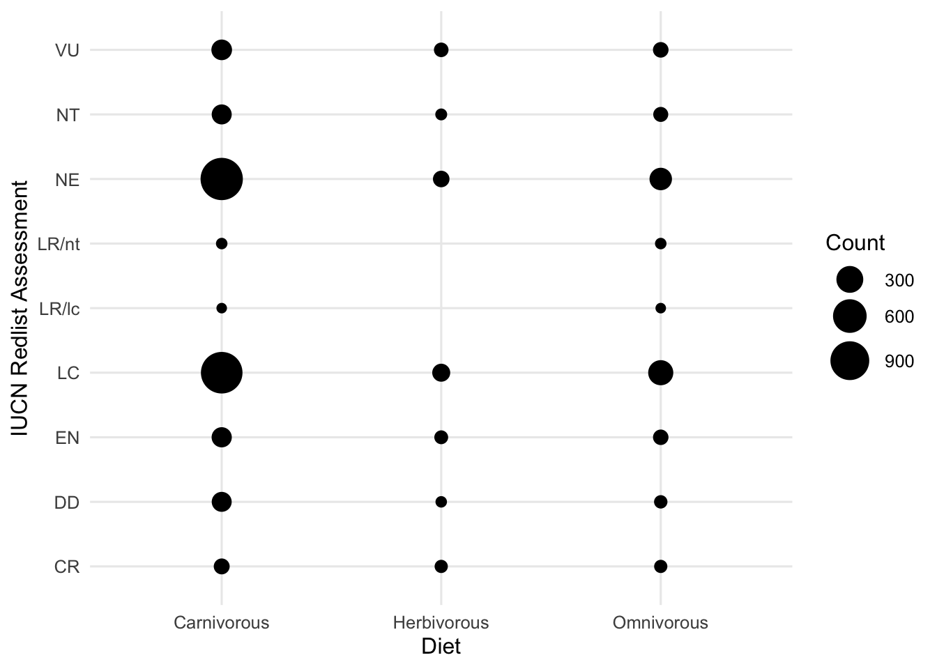
Based on this, you may ask yourself what variables/relationships you want to explore further and which you could possibly remove from your dataset.
Outlier Detection
Remember those really long species? Let’s look at them a bit more closely! But this time, we will group by family and highlight outliers using the outlier arguments available in geom_boxplot.
# Boxplots to show distributions of maximum SVL by family
ggplot(data = dfTraits %>% filter(!is.na(maximum_svl))) +
geom_boxplot(mapping = aes(x = family, y = maximum_svl),
outlier.color = "red") +
coord_flip()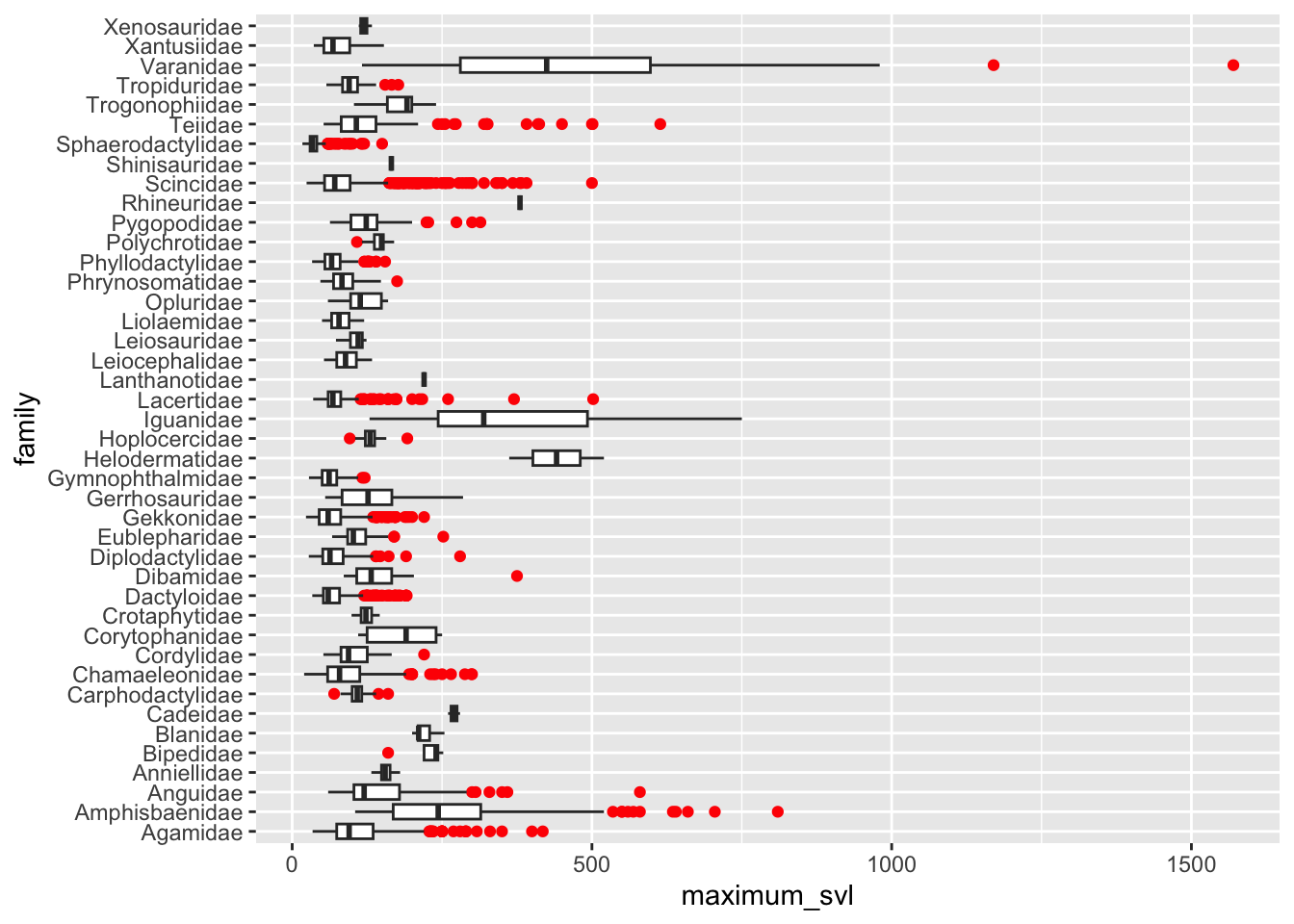
You can see the outliers are a part of the Varanidae family.
# Using the interquartile method to identify outliers.
# Determine the 1st quartile using the quantile function.
quantile(dfTraits[, "maximum_svl"], na.rm = T)## 0% 25% 50% 75% 100%
## 17.0 55.7 75.3 104.0 1570.0lowerQuantile <- quantile(dfTraits[, "maximum_svl"], na.rm = T)[2]
# Determine the 3rd quartile using the quantile function.
upperQuantile <- quantile(dfTraits[, "maximum_svl"], na.rm = T)[4]
upperQuantile## 75%
## 104# Calculate the IQR by subtracting the 1st quartile from the 3rd quartile.
iqr <- upperQuantile - lowerQuantile
# Calculate our upper threshold ((3 x the IQR) + upperQuantile).
upperThreshold <- (iqr * 3) + upperQuantile
# Identify outliers based on whether they exceed the upper threshold.
outliers <- which(dfTraits[, "maximum_svl"] > upperThreshold)
# Subset the outliers with taxonomic information.
dfOutliers <- dfTraits[outliers, c("family", "genus", "species", "maximum_svl")]
head(dfOutliers)## family genus species maximum_svl
## 106 Scincidae Acontias Acontias gracilicauda 260
## 111 Scincidae Acontias Acontias meleagris 295
## 115 Scincidae Acontias Acontias percivali 257
## 116 Scincidae Acontias Acontias plumbeus 500
## 117 Scincidae Acontias Acontias poecilus 382
## 242 Iguanidae Amblyrhynchus Amblyrhynchus cristatus 560Detect points that may be need to be ed out further. Should you remove them or not? E.g., look further into whether they might be human error or a legitimate biological observation! And of course, the choice to remove outliers will also depend on the model you end up using.
Dimensionality Reduction
If you have a high dimensional dataset, you may think about using PCA to make your data more manageable.
Principal component analysis example.
##  [1] "species"                   "genus"
##  [3] "family"                    "main_biogeographic_realm"
##  [5] "latitude"                  "insular_endemic"
##  [7] "maximum_svl"               "hatchling_neonate_svl"
##  [9] "leg_development"           "activity_time"
## [11] "substrate"                 "diet"
## [13] "foraging_mode"             "reproductive_mode"
## [15] "smallest_clutch"           "largest_clutch"
## [17] "age_first_breeding"        "iucn_redlist_assessment"
## [19] "iucn_population_trend"     "log_hatchling_neonate_svl"
## [21] "log_age_first_breeding"
# We need to remove NAs before doing this (but don't worry, we will deal with missing values this afternoon)!
dfPCA <- as.data.frame(na.omit(dfTraits[contTraits]))
# Perform PCA analysis using prcomp.
pcaRes <- prcomp(dfPCA, center = T, scale = T)
# Standard deviations for each principal component.
pcaRes$sdev## [1] 1.6122257 1.1844751 0.9899865 0.7776832 0.5604074 0.3143660# The columns here are eigenvectors that correspond to each principal component, tells you how much each variable contributes to the component
pcaRes$rotation## PC1 PC2 PC3 PC4
## latitude -0.06534507 -0.2630789 -0.94506001 -0.14425519
## maximum_svl 0.56598861 0.1275942 -0.13916457 0.34929400
## hatchling_neonate_svl 0.52114614 0.3287476 -0.12863572 0.31080620
## smallest_clutch 0.31513640 -0.5967449 0.26188578 -0.29760116
## largest_clutch 0.40091774 -0.5478159 0.03535006 0.08441005
## age_first_breeding 0.37914065 0.3875919 -0.03337456 -0.81540919
## PC5 PC6
## latitude -0.11056817 0.01860709
## maximum_svl -0.02582579 -0.72203640
## hatchling_neonate_svl -0.28648279 0.65200589
## smallest_clutch -0.62168772 -0.03063215
## largest_clutch 0.69237714 0.22671986
## age_first_breeding 0.19787267 -0.02941600## PC1 PC2 PC3 PC4 PC5
## 5 -1.277826741 -0.4472862383 -1.0958707255 -0.023995115 0.168222539
## 7 -1.259683916 -0.6764409787 -0.9883394137 0.098568843 -0.279953819
## 9 -1.147279583 -0.4949261722 -0.7168664307 -0.090289599 -0.192475942
## 22 0.150771971 0.5781564425 -0.4946526657 -0.991001796 0.612947806
## 53 -0.653580709 -0.6513218385 -0.5988712764 -0.152628583 -0.374492168
## 56 -0.919430845 -0.1379941277 -0.5472989749 0.334414105 0.108776309
## 59 -0.805705150 -0.1978411549 -0.7127529783 0.144478711 0.243969470
## 60 -1.278424339 0.0008305589 -0.6508764593 0.320326644 -0.244054779
## 61 -0.910484964 -0.2195549870 -1.0392571726 0.213150397 0.035936371
## 78 -0.486987241 -0.0338655319 -0.7446133075 -0.558469351 -0.096497581
## 81 -0.758758379 0.2201330846 -0.6485615808 0.260537749 -0.165355702
## 83 -1.148660899 -0.1776018923 -0.5403909698 0.434130563 -0.012033892
## 105 0.640244712 1.8581150478 0.8664701661 -0.101393271 -0.246736845
## 108 0.671452491 1.6584988264 0.7620965030 -0.116222321 -0.055781286
## 129 -0.407868320 0.7163980175 0.0073893518 0.578751427 -0.351791132
## 162 0.264011020 -0.9573448264 0.2092278230 0.302099526 0.499605693
## 171 0.736656041 -0.9002496377 0.7445303864 -0.282289357 -1.455657887
## 180 0.306632730 -1.6787654462 -0.3100362016 -0.146699887 -0.112472137
## 187 0.200507816 -0.7829374867 0.7213205575 -0.242807850 -0.533115850
## 192 0.473671761 -1.0321036293 0.9242670614 -0.426936919 -1.302956628
## 216 -1.181453185 -0.3216668649 -0.9745189675 -0.095493204 0.176086129
## 226 -1.476658972 -0.1240863236 -0.9991074726 -0.204268949 -0.115570345
## 228 -1.498280847 -0.2025386651 -1.2497501809 -0.244911207 -0.135579275
## 230 -1.647402256 -0.2873460883 -1.0699027415 -0.030413164 -0.157573166
## 236 -1.052951005 0.2271777831 -1.1446064778 -0.820477409 -0.004954233
## 242 3.565051335 2.6375086173 -0.6911104353 0.868874521 -0.602943005
## 244 -0.111379886 0.2413926806 0.3992373055 1.127550094 0.180502708
## 269 -0.183191452 -0.1709335775 1.5486810607 0.542262233 -0.027375168
## 270 -0.259392059 0.0872129835 1.6025311154 0.336321983 -0.190279879
## 386 -0.159523223 -0.1361619571 -0.8994936235 -1.609339363 -0.045697507
## 407 1.918418130 -1.0384145690 -1.4427335124 -1.024067174 0.045250527
## 408 1.358029000 -0.6337184941 -1.6485992756 0.088740224 0.731222653
## 418 0.312173209 0.8194694000 -1.2344733249 0.004442298 -0.334738628
## 420 -1.443654475 0.0240875644 -0.3039635485 0.340502860 -0.205042440
## 451 -1.313705760 0.0806478267 -0.0195571635 0.584518865 -0.194503419
## 464 -1.219061423 0.1067067828 -0.4911788079 0.015198484 -0.091032423
## 473 -1.437087493 0.1915696772 0.3735954139 0.490117714 -0.152130807
## 491 -1.439817261 -0.1858191610 -0.8125923040 0.418863527 -0.254904648
## 513 -1.356519847 0.0635641497 -0.3407827696 0.355580993 -0.221011138
## 517 -1.605349981 -0.0559757636 -0.1140299174 0.476064606 -0.193986275
## 536 -1.465387747 0.0160673418 -0.4856828789 0.089644862 -0.165866296
## 545 -0.356337223 0.5218927043 -0.7041927446 0.767634563 -0.510503481
## 563 -0.787424067 0.3899216235 -0.1057700235 0.813824211 -0.367216007
## 569 -1.052811441 0.0775409014 -0.4133300092 0.708700806 -0.274238309
## 571 -1.084708971 0.3913011658 0.2713838916 0.217480876 -0.083124975
## 585 -1.404186319 0.0621194925 -0.3183127286 0.147897284 -0.128619376
## 594 -1.593592399 -0.0547624684 0.0501425953 0.415577492 -0.091498291
## 629 -1.649685820 -0.1229562119 -0.0315259077 0.443848506 -0.100667884
## 631 -1.436965377 0.0056907036 -0.3243131392 0.415014417 -0.227652348
## 634 -1.354983252 0.0955326292 -0.0143880918 0.738418569 -0.303196578
## 642 -1.115606358 0.3410713947 0.0079930896 0.148368742 -0.116610477
## 643 -1.310836863 0.0799975008 -0.4780125472 0.332360615 -0.266643458
## 684 -1.459074619 0.0303353125 -0.4015322363 0.103281521 -0.144474102
## 694 -1.319535232 -0.0181696363 -0.2543584917 0.628871676 -0.215664840
## 727 -1.310330933 0.1371949050 0.0069307853 0.768284237 -0.330306069
## 730 -1.555306832 0.0102458311 0.0273982912 0.501305370 -0.185367291
## 732 -1.206989662 0.0680757830 -0.4755996321 0.241919454 -0.148521055
## 761 -1.180057758 0.1719038648 -0.2296138722 0.169579357 -0.098154107
## 770 -1.341884786 0.0331504627 -0.4765237784 -0.060151293 -0.035266522
## 814 -1.402535164 0.1459398227 -0.0310196178 0.251200855 -0.144843401
## 855 -0.415674297 -0.3612440345 -0.8387665949 -0.883070149 -0.281986353
## 917 -1.009267061 0.1305556031 -0.3536749127 0.279196254 -0.087978375
## 919 -1.047419179 0.0484066151 -0.3300906949 0.619311774 -0.182722704
## 921 -0.683716660 0.0065197961 -0.9051734384 0.312018233 -0.058633287
## 924 -0.693141398 -0.0548897307 -0.7710255450 0.380407734 0.023579266
## 926 -1.066300208 0.0296408362 -0.7315714809 0.129308579 -0.109272451
## 927 -0.888383324 -0.0177343953 -0.7772133122 0.282090934 -0.070255912
## 929 -0.815061611 -0.0247410227 -0.7201600869 0.321205267 -0.022338092
## 930 -0.730703513 -0.0965366439 -0.4590609821 0.594108713 0.072054704
## 931 -0.722341848 0.1317204634 -0.8472878574 0.248474082 -0.141266809
## 937 -0.907548126 0.0617684475 -0.9352013664 0.279143125 -0.223076516
## 945 -0.741983368 0.1107677145 -0.6817762907 0.399959575 -0.126911562
## 946 -0.833825546 -0.1654949453 -0.9877562678 0.267120220 0.017639509
## 949 -0.448567128 0.1071198307 -0.9704582048 0.294093102 -0.065081569
## 950 -0.665371388 -0.1360788233 -0.9816371986 0.520559040 -0.036175487
## 951 -0.933629616 -0.1342134553 -0.8672586866 0.230867411 0.008469735
## 956 -0.683996596 -0.1992426114 -1.0326224612 -0.857978138 -0.007337118
## 966 -1.277349658 -0.0358255708 -0.7984700814 -0.033815189 -0.099224156
## 1005 0.532653344 -0.3928848962 -0.0902934800 0.856483255 0.377867635
## 1007 0.944338124 -0.6024636915 -0.0680175895 -0.009634179 -0.106769783
## 1008 0.194476959 -0.5575175969 -0.3582815874 0.929127835 0.215536212
## 1009 -0.230027192 0.4571171252 1.6753245421 -0.329805597 0.478098159
## 1027 2.101063819 2.1423812295 -1.2837681586 -0.395420866 -0.572208004
## 1028 1.970837300 2.1240793883 -0.9750092181 -0.442787561 -0.458462988
## 1029 0.435772558 1.0406351048 -0.6549185453 0.359774310 -0.429132047
## 1040 1.431653942 1.7010908534 -1.5824505583 -0.172318434 -0.711819155
## 1043 1.878434674 1.5973465422 0.5620166380 -0.112696297 -0.815922041
## 1044 1.053786810 0.9159964344 0.5900665628 1.269506843 -0.562012237
## 1046 1.429183451 1.7776408560 0.3970717863 0.426317692 -0.215139591
## 1101 0.876466770 -2.1253022173 2.4512598150 -0.961998363 -1.148801173
## 1107 -0.453691659 -0.5929254468 1.5062400331 0.752609488 0.784749282
## 1109 0.667248176 -2.1251137690 2.5824936893 -1.202293909 -1.739326441
## 1111 0.353246520 -1.3605360680 1.8146001897 -0.672762552 -0.566053717
## 1112 0.230887988 -0.7312132102 1.7327666523 -0.176916057 0.478293923
## 1114 -0.418385639 0.2330221846 1.1724753520 0.245859524 0.104879906
## 1115 -0.745289079 -0.1877156348 0.7378060689 0.715700948 -0.063426347
## 1152 -1.140171084 -0.0906443385 0.9472675857 0.470279310 -0.144633985
## 1183 -0.626683276 -0.4878048805 -0.8853494451 0.388898055 0.418511838
## 1196 0.103557825 -0.2540160462 -0.2672027505 -0.559523591 -0.041147275
## 1208 0.312463993 -1.7977945259 0.4210213997 0.037775941 -0.427848397
## 1213 -0.085759232 -1.2629057009 -0.4313698865 0.758579669 1.452536057
## 1239 3.827327513 -5.1501487453 2.4206278219 -1.070790839 -0.671714673
## 1258 -0.772255454 0.7191047051 1.5784573091 -0.412630930 0.621129565
## 1261 -0.256935824 1.2582820574 1.7224132525 -0.926538135 0.667721399
## 1262 -0.403423629 1.0154026191 1.6858052563 -0.155401572 0.437397777
## 1297 -1.013245289 0.2169461361 1.0069295534 0.344013858 -0.288400540
## 1299 -1.092299993 0.1890259321 1.0427039450 0.261902006 -0.245661337
## 1304 -1.209729629 0.1071857769 0.9400841734 0.176301753 -0.229261242
## 1344 2.538451953 -1.8458624545 0.0932422176 -1.220510230 -0.111115502
## 1370 0.805508640 -0.5805538609 -1.1397553815 -0.086700149 0.028597847
## 1375 0.242348168 -0.2473311773 -0.8651709539 0.384421566 -0.686576284
## 1376 0.995263541 0.0388685725 -0.6519717622 -2.154587116 -0.599061107
## 1382 0.037571295 0.8379964319 -1.0115272390 -1.026374770 0.101013895
## 1384 0.374052004 -0.3784933087 -0.7053682655 0.111659142 1.021936607
## 1392 -0.187352394 0.1678646313 -0.6999908601 -0.509313102 -0.147289667
## 1399 2.832228661 -5.2052037965 1.2978208686 -0.937664825 -1.018138365
## 1403 3.525515245 -6.2079594536 0.8981103420 0.194843742 2.208458557
## 1404 0.871470087 -2.4708083417 -0.5527846957 0.617454269 1.774485348
## 1405 1.921957032 -2.8501274812 0.7516593730 1.133024299 3.613254311
## 1409 0.697863840 -1.8654419313 1.6830503030 0.515004514 0.127399664
## 1411 1.583518877 -3.7723590286 0.6819196324 0.347084024 1.378714941
## 1431 1.699497422 -0.2651100659 0.9227892008 0.205393989 0.257395394
## 1432 -0.574818920 0.8719896169 1.1201820471 0.595869350 -0.113558949
## 1439 -0.910619471 0.8998453620 1.4794630475 -0.442743101 0.360475202
## 1581 -1.000514499 0.0977473689 0.1142054648 0.613491538 -0.004969092
## 1600 -1.152644807 -0.0058494308 -0.7047141233 0.005881193 -0.044130051
## 1601 -0.622320503 0.3245151451 -0.4648228904 0.438983603 -0.206448370
## 1606 -0.271153169 0.4922556284 -0.7692131873 -0.937033233 -0.321738678
## 1607 -1.145234784 0.0580995113 -0.8611544900 0.164688369 -0.245486715
## 1630 5.828750602 1.5234604082 0.2876054896 -3.572816650 -1.799010981
## 1631 5.642031134 1.4100664831 -0.0094597721 -2.379497006 -0.501912902
## 1641 -0.875487629 -0.3925457936 -0.7412847717 0.215380225 0.349905431
## 1653 -0.178918783 1.3048908489 1.2890897756 -0.450944536 0.246156716
## 1655 0.026350200 1.3728217970 0.9586627350 -0.805594216 0.308902421
## 1672 -0.478274014 0.8648495341 0.9125945892 0.634624367 -0.162794847
## 1674 3.117503495 2.8084724633 -0.4257911444 1.881289058 -1.468235698
## 1679 -0.049790315 -0.1681146377 -0.0955977790 -0.611173841 -0.103117115
## 1683 -1.424228608 0.4860783025 1.4764114274 0.099435870 0.231488577
## 1688 1.646884544 0.9814184349 0.0814239372 0.534693333 -0.828776076
## 1689 -1.231823965 -0.0369496986 -1.1408465868 -0.064686864 -0.202239452
## 1692 -0.556686642 -0.3209354746 -1.1179307167 0.519241776 0.127048101
## 1693 -0.033329148 -0.6990943314 -0.9272756246 0.601477745 0.786639717
## 1698 -0.058230168 -0.8505733479 -0.4509122827 0.127894980 -0.621527888
## 1757 -0.731236938 0.0218007592 1.2082997456 0.429597334 0.092760913
## 1764 -1.091484200 0.4295717826 1.3834719878 0.547367588 0.186683136
## 1766 -0.974108598 0.3424572430 1.1193961045 0.616437769 0.188772901
## 1767 -0.744313841 0.3462948854 1.4453297425 0.267620034 -0.061465006
## 1768 -0.928564148 0.5257415856 1.3128308297 0.497899434 0.169605317
## 1772 -0.445415930 0.3022353574 1.1557267000 0.630020597 -0.158969665
## 1773 -0.524167132 0.3593677162 1.4289115032 0.608392841 -0.136944312
## 1794 1.432575969 0.3043007782 -0.4076779722 0.118768426 -0.939590111
## 1796 4.210929362 -2.9374717339 0.2643322379 -1.006578223 -0.241076881
## 1798 5.418836135 -5.1179203106 0.6171777032 0.158888425 1.385150435
## 1845 -0.604571056 0.4084159029 1.4286848933 0.354450898 -0.098102835
## 1870 -0.853797161 0.6158503681 1.2454710161 0.479173105 0.103443929
## 1873 -0.103517557 0.0446817394 1.2858090490 0.386267304 -0.234110010
## 1890 -0.380871885 0.8351341982 1.1434954034 -0.213589942 0.419969264
## 1904 1.393024052 0.0622177261 0.9473795723 0.685811472 1.539192791
## 1910 3.653212323 2.3881541059 -1.2056700036 -1.626439159 0.028700649
## 1912 4.610727544 0.5373433445 -0.9119968447 0.765686850 -0.735579960
## 1913 6.479721712 4.3736363770 -1.7272466760 -5.018558746 1.639206028
## 1914 3.551699329 1.4353384751 -1.2481866923 0.948871302 0.272110767
## 1915 4.467465805 0.7449951085 -1.3835199812 2.065197232 0.177570491
## 1916 4.617183757 0.3790438518 -0.6222900482 -0.447821201 -1.205700829
## 1917 2.953074241 0.5895556121 -0.9537619703 1.226740072 0.106556638
## 1919 4.998253212 1.6276284389 -0.8843773983 -1.528100840 -0.493061241
## 2073 -0.466263393 0.5372821898 0.8531177986 0.418469874 -0.430769233
## 2094 -0.993383233 0.2829779659 -0.3673150061 0.169843379 -0.178359248
## 2152 -0.772574833 0.5882955983 -0.2117730371 -0.541111231 0.052072597
## 2175 -0.224460434 0.6271504490 0.7505359894 0.560665661 -0.504673350
## 2225 -0.364986701 0.4339984811 -1.2274201755 -1.329932960 0.348384104
## 2230 -0.656579025 -0.1360869612 -1.1074092123 -0.835770962 -0.098307743
## 2234 -0.359940126 0.2503577740 -1.0976269953 -1.502164250 0.004233559
## 2236 -1.101056962 -0.3301940782 -1.1550180670 -0.064015067 0.134940317
## 2241 -1.074559846 -0.3831613270 -1.0413976292 -0.197856284 -0.349416401
## 2245 -0.998852169 -0.1942764708 -1.0786373590 0.022065221 0.045567296
## 2246 -0.283618936 0.8199470770 -1.2031705019 -2.103409349 0.406083037
## 2249 -0.561541007 -0.1201683945 -1.1844806906 -0.783352345 -0.119388562
## 2252 -0.266293798 0.3122127080 -1.2098308826 -1.305936474 0.508359501
## 2254 -0.024192734 0.0142744503 -1.0580278392 -1.379353671 0.353250499
## 2275 -0.333522431 1.2425673662 1.4405870685 -0.084921728 0.115211298
## 2326 -0.211705938 0.1175794536 -1.1707850612 -1.455994683 0.154977434
## 2332 -1.100091350 0.5650465227 1.1222734474 0.409166344 0.011201912
## 2351 -1.112667186 0.2357933987 1.3465655285 0.390422866 -0.235522681
## 2394 -0.975450887 0.3505615645 1.1729270399 0.282819352 0.365493513
## 2396 0.444774595 0.4717614696 -0.9487880849 -0.728292494 -0.118051726
## 2447 -0.796082891 -0.2246025809 -0.1584055086 0.409840095 -0.279269056
## 2452 -0.924804864 0.1507965421 0.5268448153 0.606169700 0.153184483
## 2465 1.913033954 2.2095051851 1.0222150928 -1.432624561 0.798388687
## 2472 1.127399434 1.7747555915 0.5533932269 -0.183114790 -0.013322922
## 2473 1.716029169 1.5095920066 1.0653797383 -0.035667681 0.034842115
## 2480 2.072460386 2.5149840358 0.7178161040 -1.330801639 0.372613350
## 2481 0.304050868 0.9728991803 1.1743487779 0.017034249 -0.145096373
## 2485 0.216602776 -0.1998821463 -1.3379229796 -1.006614578 0.390722759
## 2487 0.720534064 -1.3025026701 -1.0656767415 0.223373009 1.877492245
## 2495 -0.932565215 0.3442204576 0.2148220843 0.475851776 -0.105373762
## 2509 -1.242590905 0.3810727340 0.7899365013 0.356035727 0.006204751
## 2515 -1.279209769 0.3676893667 0.7431013267 0.326925430 -0.010276410
## 2598 -0.728281758 -0.4612700642 -1.4058308191 0.235205171 0.193845344
## 2612 -1.283384437 -0.1230507558 -1.0975858503 0.037831511 -0.182515044
## 2614 -0.735961692 0.1924413849 -1.2142201127 -0.667753991 0.083323703
## 2618 0.174410142 0.4806441431 -0.8714050093 -1.613765681 0.200517859
## 2619 -1.004869683 -0.4447244398 -0.9712647819 -0.173209352 -0.240167290
## 2622 -1.114842390 -0.0573742102 -1.0183803483 -0.004648372 -0.104924349
## 2624 -0.647704625 -0.7629261042 -0.9250710366 0.167160150 0.093693256
## 2628 -0.787373822 -0.3763149036 -1.1009161401 -0.049209059 -0.307622346
## 2643 -0.231664007 0.7716490507 1.0720912106 0.077702168 0.391168018
## 2648 0.988632872 0.9314364501 -0.8545425013 1.077611963 -1.133414688
## 2650 -0.154557501 0.5395251288 -0.9605487737 0.549069468 -0.442523097
## 2660 -0.440953092 0.9854538158 1.3881155005 -0.198253298 0.341968937
## 2661 0.186346337 0.6409587702 1.2582969675 -0.099147299 0.220072001
## 2662 -0.126408775 0.9389562568 1.4670820334 -0.044960291 0.498322758
## 2669 1.075221610 0.0387156777 -1.0571271222 -0.358278290 0.379221622
## 2678 -0.812533327 0.4877626772 1.1378573901 -0.202304933 -0.129846510
## 2680 0.743746399 0.2997882493 -0.7903270272 -0.593711272 -0.463001728
## 2717 -0.353533776 0.1170231275 -0.3554665943 0.541149574 0.125704116
## 2754 -0.342763814 -1.5399390792 1.4499243411 0.461056629 0.536309343
## 2756 0.140011063 -1.7947497812 1.7686957683 0.198267374 -1.339062959
## 2757 0.069339712 -1.2077294700 1.3126669844 0.819801024 0.198436979
## 2761 5.980164620 -8.8152760362 3.9421682818 -2.077032355 -4.230125507
## 2762 2.387761472 -3.5567680564 1.6980408503 0.381080573 0.022022034
## 2768 2.607516864 -4.2162796493 2.0807949941 0.240727774 0.344208964
## 2771 -0.472246975 0.3589334123 -0.8030139428 -0.469156282 0.136415298
## 2772 0.428467539 0.3225937086 -0.8468555237 -0.145963055 -0.204099961
## 2773 -0.445660786 0.4284753776 -0.8010253674 -0.366871094 0.032123008
## 2774 0.058568237 0.1257389971 -0.7553173373 -0.384835332 -0.056940177
## 2776 2.080595026 -0.0348285099 -0.9079449849 0.403397424 -0.581751946
## 2777 1.797654611 -0.0909020869 -0.7716795583 -0.600866036 -0.154963494
## 2779 -0.189950106 0.4088374448 -1.1565738432 -0.042147753 -0.139476178
## 2780 -0.171238624 -0.2155843348 -1.1012176728 0.665181009 0.152404488
## 2818 -1.506778505 -0.1316217340 -0.0500335184 0.662978358 -0.137685824
## 2835 -0.862371849 0.8484545611 1.2799703384 -0.145999062 0.197951714
## 2854 -0.163555766 0.5385501535 -0.4510006987 0.891549840 -0.375890717
## 2906 1.332304769 -1.4984926882 -0.3711607341 -0.479133506 0.366164099
## 2944 -1.541447218 -0.0194762229 -0.0055253054 0.369725135 -0.103110529
## 2947 -1.438500186 0.1789979433 -0.0781785802 -0.066437625 -0.063661594
## 2957 -1.356072640 0.2937108852 0.5117415546 0.037104886 0.070169639
## 2974 -1.496706738 0.0921469090 0.0192614461 -0.033324889 0.017334069
## 2976 -0.257924611 0.6980379581 -0.7072979425 0.161900884 -0.358585993
## 2979 -0.586482891 0.1797820277 -0.3779964026 0.208195748 -0.568445112
## 2982 -0.715757883 0.0315931774 -0.6269642796 0.100423623 -0.537939721
## 2999 0.218027653 1.0062071976 0.1479095459 -0.808376027 0.441115399
## 3028 -1.453760397 -0.0541999357 0.0424928082 0.258895640 0.046883725
## 3046 5.354521215 2.7668874619 -1.4132806282 -1.624075540 0.373028196
## 3047 3.381391190 2.0445589157 -1.7668940739 1.034047568 -0.750009558
## 3061 -1.287783155 0.1532958713 -0.0230430633 0.239272208 -0.083315716
## 3075 -1.209770421 0.0284633932 -0.5294920455 0.075851186 -0.057237433
## 3091 -1.073288889 0.0813248169 -0.5775847616 0.228830801 -0.136119543
## 3095 -1.476913879 -0.0423613518 -0.0726306308 0.584339456 -0.179100563
## 3097 -1.456406058 -0.0510083982 -0.1045243248 0.701872802 -0.233572316
## 3111 -1.202855216 -0.2170830549 -0.4600639867 -0.044120700 -0.400118475
## 3136 -1.098334145 0.3741565920 0.4132008769 0.262401817 -0.023616121
## 3164 -1.205733773 0.1989819304 -0.2029597309 0.054233345 -0.074535185
## 3193 -1.283413451 -0.0712409534 -0.7541977802 0.177117135 -0.150434971
## 3203 -0.526158785 0.8706983514 1.3854211707 -0.265280967 0.443232117
## 3231 -0.238645114 0.6385630432 -0.3061214483 0.639672481 -0.345776223
## 3233 -0.301047931 -0.0677549278 -0.9175429409 -0.471728449 -0.077617778
## 3235 -0.858839065 -0.3228612593 -0.9845203885 0.226173813 0.184108639
## 3236 0.106420498 1.3856157514 1.4361566811 -1.772361505 0.353981592
## 3241 -1.298808839 0.4516876801 1.1980780290 0.364926489 0.078465932
## 3244 -1.160562286 0.1872275803 1.2056649899 0.236811777 -0.195233591
## 3250 -0.985815643 -0.4678570134 -0.8422779176 0.112829224 0.372986159
## 3251 -0.928461260 -0.3866868424 -0.5744746376 0.049108965 -0.200441594
## 3255 -0.560772338 -0.0691730419 -0.1977087055 1.006418395 0.044794976
## 3259 -1.062616203 0.0972812344 -0.0656178766 0.710532937 -0.171320122
## 3266 -0.544370266 1.4168890444 1.7692571547 -1.035989137 0.447567618
## 3281 1.316596726 2.3786742055 1.4781254555 -2.723889250 0.495657104
## 3304 -0.694518585 -0.1112770590 -1.1271924644 -0.776335499 -0.178681071
## 3305 -0.796769024 0.2175431258 -1.2468919121 -0.624953514 -0.010903766
## 3306 -0.883741157 0.1617904028 -1.2286239378 -0.677165590 0.036605955
## 3307 -0.788996078 -0.5705545042 -1.0377064456 0.061235095 -0.149584829
## 3309 -0.670579953 -0.0909696375 -1.3229725729 -0.705666283 0.355309817
## 3310 -0.126397013 -0.1979073310 -0.8632514016 -1.747753670 -0.550860902
## 3311 -0.815940517 -0.6480018894 -1.0950838273 -0.047601358 -0.059918943
## 3313 -0.767392239 -0.6108361582 1.1316439775 0.344331769 0.019506994
## 3318 3.248779146 -0.0331118047 -0.5507165424 0.076670763 0.252687680
## 3319 5.425173126 -3.0745594344 0.6065078252 1.037798636 0.988919817
## 3324 1.233011107 -0.2651683298 1.2284618474 1.028508065 0.419071810
## 3346 0.244266791 -2.3247412689 0.1389559884 -1.316395004 -1.414354357
## 3359 -0.878533743 -0.4038937075 -0.4189025817 -0.029334522 -0.042480728
## 3411 -0.424099405 -0.8682255069 -1.5461901291 0.147946756 0.721053654
## 3413 -0.093376562 -0.3855993576 -1.1399875953 0.153169445 0.601208549
## 3415 0.354479005 -1.4470576918 -0.8816045237 -0.265784883 0.162286242
## 3416 0.134484835 -1.2286769878 -0.9146453557 -0.024127401 -0.277498648
## 3418 0.371813441 -1.5493504227 -1.0527601250 0.016632605 0.064865233
## 3426 0.576823607 0.0058051707 -0.4070171618 -0.261651323 -0.252344481
## 3429 -0.615485324 0.3075321451 0.0907627363 0.622130796 -0.038551321
## 3436 -1.066379959 0.2931901848 1.3771191421 0.234194308 0.484360582
## 3438 -1.200736531 0.3347714674 1.5388868543 0.482667129 0.324357098
## 3492 -0.643094754 0.4296796408 -0.5730693174 -0.078208991 -0.109066507
## 3552 -1.627627298 -0.2009880349 -0.0753598423 0.583866334 -0.104008825
## 3697 -0.168628746 1.0987114126 1.1979490008 -0.047774300 0.210990834
## 3739 -0.144090431 -0.3614593994 1.5428876481 -0.292876843 -0.748252249
## 3861 -0.839461983 0.5805178691 1.0487682227 0.394914583 0.104684195
## 3904 -0.006173191 1.2183342350 1.5837179441 -0.809094374 0.720408940
## 3948 -0.062274067 -0.4400587770 1.3493635075 -0.274916207 -0.718523974
## 3995 -0.405996975 1.0215824355 1.1607093797 -0.188217057 0.220131875
## 3996 1.090181837 1.5629322092 0.6773425666 0.661421839 -0.185252067
## 3998 -0.071537956 1.1416146197 1.1402317903 0.006969754 0.165585778
## 4000 -0.059577658 1.4496025224 1.2937168445 -0.809004118 0.342183458
## 4005 -0.141777556 1.1327292166 1.3175684603 -0.017318133 0.230455304
## 4034 -1.176325553 0.1338713651 -0.1698929873 0.048042252 0.009048041
## 4037 -0.009799564 1.1292513218 1.4306584990 0.067034339 0.318686217
## 4047 -0.091498297 -0.4254537259 0.8372593063 0.488035734 0.650778532
## 4049 -0.189669721 0.6296912794 0.7265497544 0.731859332 0.091736503
## 4051 -0.296616029 0.2690978773 1.3465579383 0.488591875 0.100570372
## 4064 -1.365428221 -0.2534518588 0.1884950081 0.127823496 -0.253184130
## 4071 -1.415189272 0.3436920973 1.3502306090 0.742081471 0.006689978
## 4076 -0.925637838 0.3885356771 1.2770904719 0.174993776 -0.217069257
## 4077 -1.005716523 0.2901665288 1.1925866868 0.260302996 -0.237026880
## 4115 -1.518126478 0.2447222968 0.9166588822 0.268561912 0.098090698
## 4151 -1.576212237 0.0487796327 0.1606352463 0.005318542 0.067257735
## 4183 -0.367574288 0.0532562059 -0.0826513682 -0.715034849 -0.404625637
## 4235 -0.592168027 -0.2214086731 -0.1852255362 0.133176364 -0.063942580
## 4251 -1.407949029 -0.1935466365 -1.0259482961 -0.031909467 -0.106122085
## 4253 -1.246450847 0.0518006776 -1.1432667462 -0.652239749 -0.008014237
## 4255 -1.487708098 -0.1587783488 -0.9683623992 -0.062771592 -0.140389428
## 4269 -1.559233440 0.1382253228 1.2780938616 0.544429028 0.197877993
## 4272 -1.251159917 0.4120124154 1.0445949942 0.666260226 -0.078611936
## 4274 -1.077355241 0.3857630174 1.1916692684 0.607276789 0.122894783
## 4278 -0.568481830 -0.5093085170 1.1308325007 0.613312962 -0.116517574
## 4285 -1.115694360 -0.0995588288 -0.7043798804 0.002141952 0.063193294
## 4287 -1.103420461 -0.3547950279 -0.5019703700 0.268561490 0.274314594
## 4291 -1.271883897 -0.3647085290 -0.6799336896 0.241077709 0.133869027
## 4292 -1.096850825 -0.2368805130 -0.4215555192 -0.144802381 -0.266573080
## 4309 -1.531771278 0.1985214381 0.9101062554 0.476051260 0.031480696
## 4328 -0.891041354 -0.2350086051 0.5890324258 0.584715995 -0.089554895
## 4339 -0.241332521 0.6549535297 0.9669863665 0.574393235 -0.449933850
## 4358 -0.117835818 -0.0216703305 1.3011826470 0.365642020 -0.160775396
## 4380 -1.231279626 0.2197791713 1.2245051346 0.537738536 0.260468226
## 4422 -0.143854491 1.5820146845 1.7342452638 -0.801366278 0.353232767
## 4431 -0.299011319 1.0509912104 0.8593781069 0.306894962 -0.123126904
## 4432 -0.635768264 0.8880891137 1.2866428561 0.575107675 -0.081327168
## 4433 -0.725132195 0.7929818067 1.1408830292 0.503429996 -0.057778470
## 4434 -0.353764331 1.1293663625 1.0431230193 -0.140693696 0.074367129
## 4436 -1.016733594 0.6563407929 1.3916851672 0.348802668 0.122281308
## 4470 -0.660465156 0.7531927499 0.7562092286 0.501379618 -0.155139482
## 4473 -0.247510726 1.1148720125 0.6702423419 -0.115219203 -0.035000779
## 4479 -0.501936369 0.5565670551 1.0756239387 0.420986324 -0.369225000
## 4480 -0.332023955 0.8188257388 1.1466376748 -0.331540198 -0.139847046
## 4482 -0.250843001 0.9127286732 1.1989674728 -0.348159622 -0.166913886
## 4491 0.304740550 1.3583545891 1.7950120877 -0.753642536 0.136568725
## 4500 -0.083800903 1.1214805652 1.3985892652 -1.029055128 0.134669363
## 4501 0.719997855 0.9625352542 1.9145655787 -0.912620053 -0.482840796
## 4503 -0.415837860 0.8600149717 1.8235814575 -0.188274875 0.653857486
## 4509 0.018893697 0.9891680113 1.5154162396 -0.097306320 -0.091263592
## 4511 0.714380389 2.0223481791 1.6070767237 -1.166656408 0.488131428
## 4513 -0.340922819 0.7908810106 1.7270180146 0.051336295 0.595583432
## 4520 0.328491154 1.1609536164 1.4807980587 -0.798944687 0.230059676
## 4526 0.686049069 2.0134703195 1.4244397151 -1.207009810 0.409248447
## 4527 -0.337662468 0.6106444368 1.7761812637 -0.346940133 0.327642484
## 4545 0.038860196 0.5421880272 -1.0662789077 -1.234192721 -0.197062516
## 4552 1.807092435 -0.5224135262 -1.0205997871 0.405947295 -0.351043473
## 4560 -1.070021295 -0.2680897059 -0.9457778624 -0.021363765 0.160301370
## 4628 -0.853531262 0.3821924595 1.1719023402 0.210036560 -0.230692021
## 4637 -0.542704620 1.1461918695 0.9039372082 -1.142502694 0.393479741
## 4638 -0.601158321 1.1663015121 1.1587110556 -1.151114313 0.460369393
## 4656 -1.384393367 -0.0603960851 -0.0007339364 0.371280924 0.020531804
## 4660 -1.326490283 0.0060577448 0.0297264365 0.409718171 -0.028827624
## 4661 -0.921376339 -0.4595811264 0.7005544449 0.408089853 0.907349020
## 4670 -1.041358189 0.1425598791 0.6028671734 0.101186170 -0.286011936
## 4692 0.449466167 -0.3942400865 -0.9456899995 -0.296518700 -0.145997342
## 4693 1.825978893 -2.2910689330 0.0323443420 -1.833378370 -2.443416277
## 4694 0.111875964 -0.4039286973 -1.0500502026 -0.115404110 0.219184430
## 4695 0.167419372 -1.0330944896 -1.0299282504 0.452426895 0.580786004
## 4697 0.869242840 -0.3368374194 -1.1090093418 -0.083778745 -0.843027551
## 4700 -1.043295411 0.5808061581 1.0390832653 0.292393246 0.052176711
## 4706 -0.822667204 0.2890602459 0.7806069121 0.366738406 -0.373312166
## 4710 -1.113326378 0.4391268284 1.0357181706 0.826196858 -0.107818463
## 4719 -0.828655202 0.1776079151 -1.1067771072 -0.715000553 0.117197903
## 4753 -0.434947361 -0.4857397284 1.5945747373 -0.248829044 -0.111377060
## 4764 -0.299077335 0.1217621146 -0.8008578472 -0.576324091 -0.161615119
## 4767 0.639794076 -0.8733069144 -0.4246521267 -0.559059400 0.102197635
## 4772 -1.213787159 0.3812816735 0.7852084213 0.517694820 -0.063908904
## 4781 -1.376322154 0.3570147501 1.0515440845 0.300935681 0.105193214
## 4784 -1.001337631 0.6154951055 0.7584423629 -0.145616462 0.133116962
## 4787 -0.815740955 0.5724503377 0.6932970861 0.615626850 -0.127841113
## 4798 -1.310937405 0.3560245828 0.9652729580 0.476852184 0.013284213
## 4799 -0.753205754 0.6776801150 0.8556245259 0.456217046 -0.049415702
## 4805 -1.283668978 0.4172148186 1.0297373789 0.356232793 0.052549178
## 4832 -0.967982126 -0.6132741839 -0.8349434104 0.273145766 -0.213080410
## 4875 -0.798887940 0.1991358274 -1.1292364545 -0.324586504 -0.092369575
## 4876 -1.226419406 -0.2909083639 -1.3302697657 0.094422311 -0.117370171
## 4877 -0.848240645 -0.6735077676 -1.2447939272 -0.157366954 -0.066219732
## 4878 -1.395139586 -0.0460214264 -1.1234884787 -0.153213092 -0.228318854
## 4882 -0.224823095 0.1845732297 -1.3603808790 -0.414286900 0.160133767
## 4884 -1.065329537 -0.5445336998 -0.8299920677 0.007673272 -0.202234042
## 4885 -0.959101399 -0.1419958949 -1.1589146330 0.052280653 -0.030079329
## 4893 -1.130618787 -0.4895707087 -1.0025747885 -0.026165516 -0.346770023
## 4894 -1.237710359 -0.1298380303 -0.8489163157 0.225248230 -0.137824356
## 4899 0.474474982 -1.7173332266 -0.4294530413 -0.822461244 -0.380003459
## 4903 1.800587120 -3.9986651865 0.2281780689 -1.092619186 0.229111365
## 4904 1.479399587 -2.7625958050 -0.2793543561 -0.836237482 1.177332496
## 4906 -0.687699006 -0.3692945468 -0.7543507086 0.088462954 0.474141786
## 4907 0.324415302 -1.7300634140 -0.8996756698 -0.810229789 1.327754665
## 4909 1.303146145 -2.5360439178 -0.5393163490 -0.745387758 1.385230421
## 4910 -0.445959303 -0.3549680331 -0.8074320459 0.144340444 -0.132147994
## 4911 -0.179109676 -1.9992836667 -0.1428308100 -0.454422533 -0.493932791
## 4914 -0.326195625 -0.6050177326 -0.9424527320 -0.380560603 0.366266082
## 4916 1.187835275 -2.2557918714 -0.1127870213 -1.004297953 0.043259480
## 4981 -0.183716791 0.9675710576 1.4268643774 -0.207473741 -0.150797856
## 5011 1.907000638 3.3107236394 0.9287949271 -3.935023873 0.883204121
## 5018 1.186083932 2.6640427937 1.4390306626 -2.612007597 0.721235787
## 5028 1.096890102 -0.9043793666 -0.3515879599 0.132866573 0.063640491
## 5054 -0.509990309 -1.2033467494 -0.5913816804 -0.344797125 -0.343885146
## 5062 -0.593809817 0.1417708149 -0.3116317040 -0.695630062 -0.061592737
## 5066 -1.247382209 -0.4695732847 -0.7288260737 0.455095395 0.123661246
## 5068 -0.449293593 -0.9796611637 -0.8577865170 0.003439467 0.511214496
## 5072 -0.291154774 -0.5935533912 -0.6768942153 -0.636906051 -0.050848185
## 5077 0.233001513 -1.5399144815 -0.5493575365 -0.165516456 -0.371495475
## 5086 -0.329131175 -1.1428009844 -0.8688810754 0.023758733 0.706371748
## 5088 1.354148301 -1.4213709104 -0.5415517110 -1.078892815 0.502603001
## 5095 -1.033499440 -0.1304698846 -0.6108799991 -0.098588826 -0.438330166
## 5096 0.058325918 -1.0940564428 -0.7630716031 -0.938848111 0.050623991
## 5097 -0.426019029 -0.2644178390 -1.1072517043 -0.743169106 0.096348373
## 5113 -1.136330049 -0.4673421101 -1.1712794422 0.187884521 0.119883511
## 5116 -0.977023632 -0.2334529988 -1.1408673976 0.245801157 -0.042074881
## 5118 -0.936010464 -0.0764247683 -1.1179950787 0.157188264 -0.113537108
## 5120 -1.204743479 -0.2524237783 -1.1292473091 0.202755292 -0.108297594
## 5123 -1.188596614 -0.2716659860 -1.1814417043 0.279674945 -0.140604097
## 5126 -0.846066284 -0.5211076059 -1.2582147225 0.018883551 0.359373995
## 5128 -0.776088786 0.0586735030 -1.1277079434 -0.263479969 0.029899994
## 5130 -0.646095735 -0.6792778726 -1.1017861861 0.103769303 -0.026567762
## 5131 -0.489226739 -0.3840894501 -1.1641297439 -0.355761048 -0.034514433
## 5136 2.349200228 -1.9725131764 1.7198238981 -0.077716973 1.360605541
## 5139 0.620034011 0.2766918665 1.1865866670 0.048296101 0.691098953
## 5142 2.738564579 -2.2016526363 1.4851650296 0.332990190 2.784326813
## 5143 0.719168201 -1.2995981271 1.0276395364 0.620608849 0.574640946
## 5226 -0.732017680 -0.2782703262 -1.0345813773 0.069980005 0.255658980
## 5229 -1.396313021 -0.4297594007 -1.0442037041 0.294437095 -0.043634675
## 5236 -0.873971518 0.4672838015 1.6233429966 0.381884366 0.442084600
## 5237 -0.675670575 0.0543597430 1.6676668609 0.256005407 0.356684526
## 5238 -0.511981953 0.4271545129 1.7151155150 -0.476224370 0.458152444
## 5239 -0.607900569 0.9972270816 1.5261997189 -0.275589757 0.341767739
## 5277 0.205001593 1.1862701750 1.0833331205 -0.282833079 0.390832574
## 5298 2.867671389 0.7802948515 -1.7703534866 1.209715782 -0.419726720
## 5301 -0.443765047 0.8616109997 0.6455131646 0.625118451 -0.264251350
## 5307 -0.316637404 -0.8245291721 -0.3841516001 -0.145876824 -0.613509725
## 5312 -0.736267652 0.4681821718 0.8280901946 0.480574407 0.121949478
## 5314 -1.110210112 0.5904705000 1.1693144590 0.263637251 0.074449593
## 5334 -0.774320396 0.5286499230 0.1945004771 0.369716442 -0.161837718
## 5335 -0.868118152 0.3462014323 -0.3491053261 0.251312786 -0.206017182
## 5343 -0.718932643 0.4606952591 -0.8375723651 -0.575195747 -0.045860489
## 5344 -0.714356326 0.4591062845 -0.5456590910 -0.106863991 -0.147039772
## 5365 -1.052113277 0.3146756035 -0.7889230040 -0.781240838 0.042830729
## 5370 0.860495631 1.5998246784 0.6060727883 0.581864427 -0.286278282
## 5380 0.821899257 -2.0763468673 1.9474544270 -1.458477047 -1.194744608
## 5407 -1.162163106 0.5449199594 1.1677878234 0.374840710 0.034940959
## 5448 0.542600774 1.4281180223 0.9987561396 -0.664271815 -0.196449542
## 5452 5.088623817 -1.9189654281 0.9820937915 0.277594292 1.545830681
## 5453 5.449908986 -2.6059089832 1.9458848982 0.168448497 -2.403593111
## 5472 1.053813484 -0.1787295023 -0.9677483733 -0.088396808 -0.160754193
## 5480 -0.691691325 -0.4268116568 -0.2622950598 -0.216972466 0.218580062
## 5490 0.211188476 -0.4380335339 -0.7672870126 -0.206579106 0.464533663
## 5498 0.301646012 -0.6010758018 -0.7980242815 -0.128520084 1.277778161
## 5499 -0.570493635 -1.0216787738 -0.5256788499 -0.113630715 0.030763195
## 5505 0.712819242 -1.0691223975 -0.2685881162 -1.002159902 -0.058633502
## 5512 -0.248306752 -0.5346265587 -0.2434872131 -0.080375768 0.481850358
## 5513 -1.143383747 -0.0336416591 -0.3511625534 0.326389718 -0.017390196
## 5516 -0.877600402 -0.3388170070 -1.1419460092 0.052261883 0.206010775
## 5517 -0.792629067 -0.9668349267 -0.3704171791 0.386623256 0.352863324
## 5521 0.250094693 -1.5525979314 -0.1351296158 0.005792943 0.393483115
## 5526 -0.591125131 -0.8463607793 -0.5253007198 0.582461960 0.176295009
## 5534 0.158111542 -0.4853614607 -0.8011108991 -0.243220112 0.490305470
## 5535 -0.579139034 -0.2686968662 -0.1086602221 0.137008693 0.021945486
## 5538 -0.992643161 -0.4296365866 -0.5832751391 -0.063670743 -0.134101818
## 5540 -0.111480836 -0.0922852932 -0.3166759217 -0.569901109 0.343362994
## 5543 -0.228495735 -0.9699856523 -0.9100283515 -0.472045068 0.164691962
## 5545 0.870590286 -2.9959838851 0.0713271811 -0.400194718 -0.272262343
## 5547 0.466377918 -0.1629796821 -0.6480514417 -1.280439858 0.235717227
## 5551 0.364071884 -1.2839002119 -0.4299257965 -0.124913610 0.133357898
## 5555 -0.704348694 -1.0801866304 -0.2251301683 0.124219690 0.034331221
## 5559 -0.753386873 -1.0751060745 -0.4291119369 0.011733587 -0.028585550
## 5570 0.097607183 -0.6635175000 -0.3237888722 -0.280628106 0.195762187
## 5571 -0.308443230 -1.3864487479 -0.5015512320 -0.337320439 -0.688738469
## 5572 -0.454780412 -1.1409421047 -0.6878179764 0.023543887 0.067221877
## 5575 -0.682735469 -0.4569097539 -0.3080662853 0.252669608 0.005323723
## 5576 -1.169209454 -0.2363178548 -0.4258292987 0.564322023 0.015599976
## 5577 -0.539952885 -1.1748210240 -0.4517052669 -0.054434576 0.192301274
## 5578 -1.012142268 -0.5056702475 -0.5412477132 -0.012342919 -0.077627202
## 5607 -1.315902499 -0.0576140605 -0.2328692258 0.316442981 -0.022599340
## 5617 -1.270359354 -0.3295349756 -0.8463349850 0.093271175 0.106203692
## 5663 -0.843714293 -1.4312606027 -0.1299378411 -0.378174906 -0.736760587
## 5666 -0.295592846 -1.5118973703 0.3426049108 -0.167404033 0.374732060
## 5668 -0.694197427 -1.7204527683 -0.0508456879 -0.577015986 -0.916600963
## 5682 -1.715569854 -0.1232945036 -0.3542967436 0.162861350 -0.137149666
## 5703 -1.628789062 -0.0230929952 -0.2925326926 0.007474925 -0.088339735
## 5708 -1.514535328 -0.0299477073 -0.3857861006 -0.016336033 -0.053784985
## 5738 -1.841639594 -0.1675430226 -0.2225874786 0.098079050 -0.067500870
## 5739 -1.515123866 -0.0511118301 -0.3935689867 0.126687541 -0.108750547
## 5752 -1.562610846 -0.0072687716 -0.3549502552 0.114312184 -0.151571371
## 5760 -1.232156728 0.3303891993 -0.3113049455 -0.468026321 -0.011736672
## 5781 -1.372265117 0.2586831078 -0.1578415711 -0.466377251 0.057952799
## 5813 -0.678804721 -0.1677863849 0.0554168573 0.350384115 -0.149103556
## 5832 -0.989629406 -0.3804580257 -0.3521477363 0.481754160 -0.353456053
## 5908 0.609585581 -0.6824185714 -0.8377908655 -0.405250632 0.326192942
## 5979 -1.143311248 0.0988670414 -0.5708785546 0.342363360 -0.245636856
## 5993 -0.097825979 1.0838235639 1.0627786192 -1.060661824 0.040124664
## 5995 -0.929063842 0.8526625002 1.2059113636 -0.485663315 0.292642125
## 5997 -0.487348216 0.8086673050 1.4465941092 -0.396914253 -0.048680553
## 6004 -0.835846786 0.8755090157 1.3730057610 -0.118627407 0.214280890
## 6005 -0.487201300 1.1530414030 1.1139666479 -0.650999507 0.263293913
## 6007 -0.480490152 0.7674478682 1.2038173499 -0.419745479 -0.101742229
## 6010 -0.701957917 0.9614703838 1.1246778510 -0.351519418 0.199549121
## 6025 -0.995781639 -0.0632883740 -0.8140293614 -0.005687036 0.049857459
## 6031 -1.104618138 -0.4170086601 -1.0076096023 0.297692159 0.101266530
## 6037 -0.643473911 0.4243659667 -0.4382005231 0.384442102 -0.265332828
## 6044 -1.319101718 -0.0151701716 -0.6399964026 0.152399481 -0.155684770
## 6055 -1.211517152 -0.0766044653 -0.9888894471 -0.047307288 -0.090232418
## 6066 -0.832495263 0.1084899840 -0.9098051524 -0.045371381 -0.061120525
## 6067 -0.261626865 0.3839753416 1.3958259463 0.599836498 -0.036407415
## 6071 -1.288064496 -0.0922426661 -1.0673046327 0.053294043 -0.198142873
## 6074 -1.158439596 0.0413292711 -1.0949540861 -0.229703058 -0.137749831
## 6075 -1.057554437 0.1663176609 -0.9076238779 -0.146918547 -0.176222028
## 6083 -0.681674702 0.2261408101 -1.3137963320 0.263183452 -0.416675883
## 6095 -0.154590486 1.1567327499 1.3011789385 0.274030881 0.044716814
## 6096 2.650871223 0.7736171796 0.0973987975 1.289502309 -1.182313728
## 6098 2.493965325 1.7570401452 0.8721064314 1.897781020 -0.180711563
## 6100 2.900646319 2.6915513686 0.4337786985 2.102382333 -1.196909904
## 6101 2.925631362 1.4665352873 0.4815201344 0.695524820 0.745750924
## 6103 0.872972068 -0.6850805237 -1.2670296801 0.225767225 0.635265917
## 6116 -1.058524382 -0.2459753281 0.2008261159 0.441413524 -0.251506802
## 6131 -0.677541570 -0.8442327359 0.2962336310 0.333430736 -0.057000787
## 6158 -0.586191592 -0.7451544856 0.5055298807 0.413919923 -0.056898912
## 6177 -0.055614718 -0.2769557316 -0.0810430509 0.188371132 0.285311541
## 6183 -0.159993950 -0.4687975727 0.6697912508 0.353191927 0.646446462
## 6189 -0.879227304 -0.1766480763 0.7273953854 0.490454435 0.625852990
## 6201 -0.075563572 -0.3411248031 -0.5572629674 -0.843094363 -0.708881797
## 6204 -0.038717095 -0.2633280679 -0.8175078431 -0.518828216 0.311062889
## 6205 0.525336094 -0.6475899409 -1.1390765192 -0.466158262 0.143655839
## 6229 1.972615480 -3.4303227829 1.5284375955 -0.274954990 -0.739871366
## 6230 -0.188131910 -1.0730847592 0.5098321041 0.644339790 0.996807636
## 6236 0.007243476 -1.4645552117 0.6355052514 0.462062657 0.293423707
## 6239 1.418827880 -2.9585613923 0.7994412276 0.656201130 1.740411676
## 6262 1.193071510 0.9603618610 -1.2591531131 -0.105503124 -0.649950101
## 6327 -0.602167269 -0.0741708332 0.8775535386 0.900792868 0.542893755
## 6350 -0.597227391 -0.5819201389 1.3839663382 0.221269795 0.236270505
## 6399 -0.860503753 -0.0238914630 -0.6752312179 0.528046664 -0.124731871
## 6401 -0.567717988 0.1409618844 -0.8902615040 0.328161953 -0.129624685
## 6402 -0.115208004 -1.9942432999 0.0868168060 -0.241127929 -1.795799119
## 6403 -0.597317056 0.1576361312 -1.0487782226 0.305038183 -0.219142385
## 6404 -0.712793127 0.7885468080 1.2705084303 0.742418340 -0.107575397
## 6414 2.895383622 -0.4019820006 -0.7997922301 -1.227760485 0.315383603
## 6415 3.326727082 -0.2663460444 -0.8604501653 -0.704678749 1.431448834
## 6424 1.028005413 -0.2701350385 -0.5781748951 -0.102806870 0.082208995
## 6450 -0.923856015 -0.6440653894 -0.7445862160 0.138569229 -0.064294910
## 6453 -0.801129429 -0.9223531514 -0.6508611583 0.110452305 0.318345225
## 6459 -0.936267522 0.0454078134 -0.7405261485 0.124959665 -0.060398029
## 6461 -1.095902257 -0.3728295414 -0.8766547251 0.173787220 0.184515303
## 6467 1.195703016 0.4378597777 0.7730731958 1.030170441 0.167951774
## 6468 6.553962670 1.1441028879 -0.3058571848 1.484845138 1.571183118
## 6472 2.402364509 2.4196839856 -0.1484513426 -0.786901488 0.031938281
## 6473 5.584764411 -0.4573560719 -1.1493591631 1.562791127 0.299518036
## 6477 -0.240534903 0.6534169130 0.9406428656 0.706686701 0.127912194
## 6480 -0.074235486 0.1674373370 1.2240181877 0.942595942 -0.642622837
## 6490 3.270663456 -0.2921534038 -0.9685862442 0.483418008 0.165584419
## 6493 0.763924594 0.4635681096 0.6933970756 1.271763518 -0.878922825
## 6496 4.482971887 -0.3321606051 -1.1174937668 1.396173746 -0.364643187
## 6498 3.266312549 1.6701180117 -0.3014681937 2.045447046 -0.883004497
## 6499 2.267581619 1.4662360660 -0.1703601581 1.479884392 -0.870311431
## 6503 10.141910469 3.8460532080 -1.6644407247 3.214740367 0.162120106
## 6510 3.685693691 1.6615549584 0.1958235332 0.929665048 -0.582100890
## 6512 5.575877161 1.2822040248 -1.1610676453 1.916377754 -0.316183331
## 6514 7.365820821 -0.6243825400 -0.5419682249 2.902272793 0.920772967
## 6517 4.727858117 1.5326222116 -1.2357107073 2.211116308 -1.146540818
## 6519 4.453115348 1.8099501598 0.1298636188 1.928045544 -0.808266821
## 6520 0.225260396 0.6033345046 0.8806481092 1.094567841 -0.463029670
## 6521 2.090859487 1.5939334949 -0.0293114262 0.309652259 -0.490431421
## 6529 6.735694547 1.3208926589 -1.6652936087 3.564318393 0.658468193
## 6542 1.890648034 0.6397109972 0.8541112846 0.625468304 -0.101879403
## 6543 5.772809058 3.5783894271 0.2181139180 -1.060587435 0.312125194
## 6554 0.214251146 1.5880037143 1.7706902728 -1.654650553 0.297325111
## 6556 0.113179344 1.8219479024 1.5854339977 -1.522053809 0.543640412
## 6563 -0.288010613 0.9311287793 -0.9554986260 -1.619209179 0.164196869
## 6565 0.286750470 0.4577600070 -0.9014387133 -1.558714167 0.243277616
## 6569 -0.671478957 0.5225506074 -0.9488573137 -1.221785604 0.183095696
## 6578 0.258152086 0.8239782281 -0.5626487267 -0.588744444 0.202965678
## 6579 0.234534536 1.0842765289 -0.7615755197 -0.862468315 -0.016800168
## 6583 0.365839624 1.0318645625 -0.7681241877 -0.807017959 0.068501844
## 6604 -0.948938030 -0.8792790468 -1.6305625933 -0.053459313 0.533947800
## PC6
## 5 -0.1133342368
## 7 -0.0777347086
## 9 -0.0770771052
## 22 0.1161075153
## 53 -0.0824282666
## 56 -0.0371975657
## 59 -0.0143610530
## 60 -0.0227393725
## 61 0.0942088107
## 78 0.0973253172
## 81 0.0546702792
## 83 -0.0817066761
## 105 0.6582654347
## 108 0.2442922549
## 129 0.2969886665
## 162 0.0700376120
## 171 -0.0017446083
## 180 0.0263451574
## 187 -0.2288134741
## 192 -0.2957969549
## 216 0.0034584440
## 226 -0.1167947988
## 228 -0.1528052015
## 230 -0.1347599285
## 236 -0.1030088556
## 242 0.0511208309
## 244 -0.1839746912
## 269 -0.0373040438
## 270 -0.0828363228
## 386 -0.1262068999
## 407 -0.2276333316
## 408 -0.0510127381
## 418 0.3130349910
## 420 -0.1975533886
## 451 -0.1156106555
## 464 -0.2504987962
## 473 -0.1274183928
## 491 -0.1666748864
## 513 -0.2073572911
## 517 -0.2189248879
## 536 -0.1764096414
## 545 -0.0812470258
## 563 -0.1859031211
## 569 -0.3258034465
## 571 -0.0187819412
## 585 -0.3348923957
## 594 -0.2103987023
## 629 -0.2457697782
## 631 -0.2093540884
## 634 -0.0752704805
## 642 -0.2589041064
## 643 -0.0790349561
## 684 -0.2366253230
## 694 -0.2593498881
## 727 0.0147823152
## 730 -0.2051792895
## 732 -0.2764643141
## 761 -0.2384486983
## 770 -0.3555715081
## 814 -0.1689890208
## 855 -0.1178199255
## 917 -0.0080155160
## 919 0.0199894112
## 921 0.1281015214
## 924 0.0413900155
## 926 0.0287572157
## 927 0.1156514873
## 929 0.1417204102
## 930 0.0733901096
## 931 0.0810073983
## 937 0.1491684169
## 945 -0.0609325372
## 946 0.1170255350
## 949 0.3343496493
## 950 -0.0407482953
## 951 0.0493597664
## 956 -0.0697602892
## 966 -0.0581935569
## 1005 -0.1988559865
## 1007 -0.3191347391
## 1008 -0.1730627269
## 1009 -0.0181201539
## 1027 1.2279420066
## 1028 1.0361335393
## 1029 0.6944743568
## 1040 1.0503732747
## 1043 0.6558965245
## 1044 0.5432382907
## 1046 0.5611811331
## 1101 -0.0497822907
## 1107 -0.0483925910
## 1109 -0.2041105314
## 1111 -0.0920862419
## 1112 -0.0040196255
## 1114 0.0924321270
## 1115 0.0607285173
## 1152 -0.0695250676
## 1183 0.0835686846
## 1196 -0.0097276455
## 1208 -0.1760182056
## 1213 0.0520749695
## 1239 -0.2904123504
## 1258 -0.1869081549
## 1261 -0.1112210249
## 1262 -0.0170538628
## 1297 -0.1013492421
## 1299 -0.1345439857
## 1304 -0.1268500402
## 1344 -0.2242963172
## 1370 0.1041531976
## 1375 0.1040570305
## 1376 0.1089767137
## 1382 0.2041234979
## 1384 0.2349246085
## 1392 0.1847577128
## 1399 0.1225215842
## 1403 0.6435640024
## 1404 0.3506874766
## 1405 0.8119626180
## 1409 -0.0090528515
## 1411 0.4879393066
## 1431 -0.1313359563
## 1432 0.0607512362
## 1439 -0.3951129549
## 1581 -0.2112301763
## 1600 -0.0614821567
## 1601 0.0960235862
## 1606 0.1072941066
## 1607 -0.0247815260
## 1630 -0.1201624977
## 1631 0.0287288657
## 1641 -0.0219846564
## 1653 0.0139928758
## 1655 0.1495387421
## 1672 0.0410736901
## 1674 2.1100365632
## 1679 -0.0341740192
## 1683 -0.2941216064
## 1688 0.1351686295
## 1689 -0.1043909633
## 1692 0.2134738055
## 1693 0.4090101899
## 1698 0.0376044453
## 1757 -0.2441416662
## 1764 -0.0071575321
## 1766 -0.0736818152
## 1767 0.0300327071
## 1768 0.0187020467
## 1772 -0.0545316258
## 1773 0.1209687498
## 1794 -0.2099808947
## 1796 -0.0496539563
## 1798 0.1036826256
## 1845 0.0151761093
## 1870 -0.0187107804
## 1873 0.0458486223
## 1890 0.0093862958
## 1904 0.1864152320
## 1910 -0.5996426783
## 1912 -0.2305251928
## 1913 -0.9499688826
## 1914 0.0339343942
## 1915 -0.6197046159
## 1916 -0.1519113883
## 1917 0.0899940231
## 1919 0.1154342601
## 2073 0.1364582888
## 2094 -0.0338583521
## 2152 -0.1498631415
## 2175 0.1147628250
## 2225 0.0159552839
## 2230 -0.0268865544
## 2234 -0.0267115572
## 2236 -0.0172349956
## 2241 -0.0505900611
## 2245 0.0169724428
## 2246 -0.1147411990
## 2249 -0.0996030909
## 2252 0.0742936569
## 2254 0.0885296463
## 2275 0.0343412473
## 2326 -0.0484538805
## 2332 -0.0638658399
## 2351 -0.1117150149
## 2394 -0.1330975246
## 2396 0.1747202976
## 2447 -0.0531596993
## 2452 -0.0766243248
## 2465 -0.0392499144
## 2472 0.6740648435
## 2473 0.4228986214
## 2480 0.6994194853
## 2481 0.4236097696
## 2485 -0.0369561103
## 2487 0.2705968457
## 2495 -0.0785624878
## 2509 -0.1695485164
## 2515 -0.0686595266
## 2598 0.1244738812
## 2612 0.0160428593
## 2614 -0.0357317231
## 2618 0.0190083898
## 2619 0.0085762166
## 2622 -0.0143413854
## 2624 0.1942327205
## 2628 -0.0306857399
## 2643 -0.0747723380
## 2648 0.6827429393
## 2650 0.2031840031
## 2660 -0.0117051056
## 2661 0.1144795574
## 2662 0.1426532791
## 2669 0.4834426961
## 2678 -0.1031314860
## 2680 0.2091288965
## 2717 0.1046195472
## 2754 0.0554999943
## 2756 -0.4328946739
## 2757 0.0217781913
## 2761 0.1057993517
## 2762 0.1342834375
## 2768 -0.0996180551
## 2771 -0.0575198286
## 2772 -0.1267911595
## 2773 0.0011533879
## 2774 0.0193656891
## 2776 -1.2413892466
## 2777 -0.7999050780
## 2779 0.3025540676
## 2780 0.3369523443
## 2818 -0.1426159979
## 2835 -0.1876524301
## 2854 -0.1937050047
## 2906 0.0593974283
## 2944 -0.1561345975
## 2947 -0.1478205805
## 2957 -0.2131883683
## 2974 -0.1871691544
## 2976 0.2748564807
## 2979 0.1759197195
## 2982 0.0322413966
## 2999 -0.3242152522
## 3028 -0.1344851258
## 3046 0.7387962796
## 3047 1.8956878809
## 3061 -0.1963860495
## 3075 -0.2333488269
## 3091 -0.1555272611
## 3095 -0.1629229965
## 3097 -0.0925166971
## 3111 -0.1003718557
## 3136 -0.2566838373
## 3164 -0.1609579083
## 3193 -0.0620867638
## 3203 -0.0797331687
## 3231 0.1599570368
## 3233 -0.0339020610
## 3235 -0.0277180546
## 3236 -0.1557700307
## 3241 -0.1871364233
## 3244 -0.1882465387
## 3250 -0.0254177312
## 3251 0.0901886082
## 3255 0.0704536583
## 3259 0.0549358504
## 3266 -0.2261841888
## 3281 -0.3236697926
## 3304 -0.0158923509
## 3305 0.0669175793
## 3306 -0.0424982999
## 3307 -0.0034043088
## 3309 0.0765634862
## 3310 -0.1151861093
## 3311 -0.0248029229
## 3313 -0.0716182328
## 3318 0.0363309680
## 3319 0.0926052887
## 3324 -0.1544260396
## 3346 -0.1649909017
## 3359 -0.1746723356
## 3411 0.1296543484
## 3413 -0.0156593920
## 3415 0.1384290310
## 3416 -0.0837999254
## 3418 0.0796617778
## 3426 -0.0054035361
## 3429 0.0602492758
## 3436 -0.1452188149
## 3438 -0.1211591998
## 3492 -0.0435451117
## 3552 -0.1659645738
## 3697 0.1540119798
## 3739 -0.1082006822
## 3861 -0.0711805704
## 3904 -0.1492801272
## 3948 -0.1676459735
## 3995 0.0751237272
## 3996 0.7618036470
## 3998 0.2132675773
## 4000 -0.0080478779
## 4005 0.0992936157
## 4034 0.0565103163
## 4037 -0.1185268546
## 4047 -0.0147252065
## 4049 -0.1097331715
## 4051 -0.1400830778
## 4064 -0.1721744089
## 4071 -0.1872288876
## 4076 -0.0386959739
## 4077 -0.0924131927
## 4115 -0.2795677459
## 4151 -0.3402549501
## 4183 -0.3770633421
## 4235 0.0709219340
## 4251 -0.1525215605
## 4253 -0.2380939916
## 4255 -0.1627613345
## 4269 -0.2431028840
## 4272 0.0241777673
## 4274 0.0644074683
## 4278 0.1373445693
## 4285 0.0052375215
## 4287 -0.0388748373
## 4291 0.0170565004
## 4292 -0.0271106530
## 4309 -0.2398819035
## 4328 0.0135024040
## 4339 0.0057500174
## 4358 0.0346205767
## 4380 -0.1213767156
## 4422 0.0132009063
## 4431 0.1830174239
## 4432 0.0907741036
## 4433 -0.0035068120
## 4434 0.0040822559
## 4436 -0.3494358930
## 4470 0.1440700741
## 4473 0.1638199118
## 4479 0.0225584570
## 4480 -0.0756111889
## 4482 0.0884153931
## 4491 -0.0011640990
## 4500 -0.0587431094
## 4501 0.2402700557
## 4503 -0.0134945430
## 4509 0.1072650181
## 4511 -0.0117214092
## 4513 0.1332435651
## 4520 -0.0548881406
## 4526 0.3013271711
## 4527 -0.0340443005
## 4545 0.1408430017
## 4552 -0.2266680699
## 4560 -0.0480097616
## 4628 -0.1365753027
## 4637 -0.2010012670
## 4638 -0.2898365415
## 4656 -0.2267475951
## 4660 -0.0368914172
## 4661 -0.0470389465
## 4670 -0.0852593611
## 4692 0.0527416404
## 4693 0.1286566391
## 4694 0.1448233176
## 4695 0.2895882143
## 4697 0.4966943505
## 4700 -0.1949065592
## 4706 0.0220291359
## 4710 -0.1230115224
## 4719 -0.0102698692
## 4753 -0.1513128046
## 4764 0.0129031059
## 4767 -0.1281264826
## 4772 -0.0653092788
## 4781 -0.3137719264
## 4784 -0.2256341115
## 4787 -0.1341639616
## 4798 -0.2031511582
## 4799 -0.1959467324
## 4805 -0.1885732870
## 4832 -0.0491716572
## 4875 0.1448006628
## 4876 0.0108869721
## 4877 0.0541370978
## 4878 -0.0700674312
## 4882 0.1050438656
## 4884 0.0115589455
## 4885 -0.0371634601
## 4893 0.0558210117
## 4894 0.0162963348
## 4899 0.0386746976
## 4903 0.2502910098
## 4904 0.5504032019
## 4906 0.0569094382
## 4907 0.2634902944
## 4909 0.4388505176
## 4910 0.1332599739
## 4911 -0.0055214782
## 4914 0.0663706395
## 4916 0.3112850539
## 4981 -0.0349015489
## 5011 0.2374200925
## 5018 0.2146475603
## 5028 -0.1354090834
## 5054 0.0189758654
## 5062 -0.0973322151
## 5066 0.0219141961
## 5068 0.1497885614
## 5072 -0.0098401910
## 5077 -0.0424020908
## 5086 0.3110896128
## 5088 0.3827625162
## 5095 -0.0300813582
## 5096 0.0334811373
## 5097 -0.0038337249
## 5113 0.0109365310
## 5116 0.0777643842
## 5118 -0.0525767832
## 5120 -0.0338377736
## 5123 -0.0307246125
## 5126 0.0826403925
## 5128 0.0536040043
## 5130 0.1270211952
## 5131 0.0830532471
## 5136 0.1099908966
## 5139 0.0672836234
## 5142 0.5677018003
## 5143 0.3600034305
## 5226 0.0456640785
## 5229 -0.0259848939
## 5236 -0.0290769469
## 5237 -0.0493665554
## 5238 -0.1676061884
## 5239 -0.0226108975
## 5277 -0.0540578975
## 5298 -0.6392910791
## 5301 0.3272441400
## 5307 -0.0603830792
## 5312 0.1095945285
## 5314 -0.1308453363
## 5334 -0.0400942579
## 5335 -0.0513116121
## 5343 -0.1436962997
## 5344 -0.0665174773
## 5365 -0.1090681787
## 5370 -0.1058886319
## 5380 -0.1161970870
## 5407 -0.0695462622
## 5448 0.1697631220
## 5452 0.2914375550
## 5453 -0.6717826216
## 5472 0.1607019309
## 5480 0.0575438780
## 5490 0.1547381683
## 5498 0.1750521746
## 5499 0.0093817945
## 5505 -0.0986048346
## 5512 0.2098960332
## 5513 -0.0586764050
## 5516 -0.0106868065
## 5517 0.0254955664
## 5521 0.1718035377
## 5526 0.1082720096
## 5534 0.0744506628
## 5535 0.0004144472
## 5538 -0.0593271704
## 5540 -0.0589048002
## 5543 -0.0012158368
## 5545 0.1361781311
## 5547 0.0782758115
## 5551 0.1387178065
## 5555 -0.0415994707
## 5559 -0.0192326455
## 5570 -0.0949250580
## 5571 -0.0859482956
## 5572 0.0643589026
## 5575 0.1100765435
## 5576 0.0044824858
## 5577 0.0858018326
## 5578 -0.0642431933
## 5607 -0.1528117667
## 5617 -0.0776393363
## 5663 -0.1711133825
## 5666 -0.0874358179
## 5668 -0.1809142689
## 5682 -0.2061805038
## 5703 -0.2183631368
## 5708 -0.1766360876
## 5738 -0.2992792501
## 5739 -0.1109104420
## 5752 -0.1340952368
## 5760 -0.1196125952
## 5781 -0.2824802599
## 5813 -0.1895275897
## 5832 0.1425004795
## 5908 -0.2903750098
## 5979 -0.0406290567
## 5993 -0.1145260807
## 5995 -0.2107171521
## 5997 -0.1263325781
## 6004 -0.2437512028
## 6005 -0.1007659083
## 6007 -0.0296587980
## 6010 -0.1023901604
## 6025 -0.0584323135
## 6031 0.0669305807
## 6037 -0.1142228178
## 6044 -0.1985176051
## 6055 -0.2658869491
## 6066 0.0940564401
## 6067 0.1023839141
## 6071 -0.2064438020
## 6074 -0.1876789745
## 6075 -0.0066129199
## 6083 0.1182171733
## 6095 0.2988075750
## 6096 1.0509803059
## 6098 0.9835162331
## 6100 1.8509645015
## 6101 0.6219509179
## 6103 -0.1621928763
## 6116 -0.1357159705
## 6131 -0.0840412573
## 6158 -0.0690908736
## 6177 -0.0607766111
## 6183 0.0912129234
## 6189 0.0170743487
## 6201 0.2318273879
## 6204 -0.1006949741
## 6205 -0.1150383261
## 6229 0.3468531214
## 6230 0.2670347029
## 6236 0.1446201739
## 6239 0.4801776599
## 6262 0.4455944713
## 6327 -0.1480868691
## 6350 0.0691966520
## 6399 0.1103645451
## 6401 0.1138382816
## 6402 -0.0127623674
## 6403 0.1707205095
## 6404 0.0068427705
## 6414 -0.5819138932
## 6415 -0.1587150656
## 6424 0.2154711989
## 6450 0.0649411115
## 6453 0.0575187262
## 6459 0.0331213664
## 6461 -0.0702533206
## 6467 0.3928259009
## 6468 -0.3614222857
## 6472 0.1738175944
## 6473 -1.6131377437
## 6477 0.2455059869
## 6480 0.3133870272
## 6490 -0.4485601698
## 6493 0.2285821533
## 6496 -0.0165537652
## 6498 -0.0318060735
## 6499 0.0232129932
## 6503 -2.4707134252
## 6510 -0.0053496661
## 6512 0.2468795281
## 6514 -0.4654193068
## 6517 -0.0050417076
## 6519 -0.6745863382
## 6520 0.2855208653
## 6521 0.5827556950
## 6529 -1.7974869301
## 6542 0.2712765535
## 6543 -1.0578445618
## 6554 -0.1228409796
## 6556 -0.1515413024
## 6563 -0.0034276062
## 6565 -0.0388880373
## 6569 -0.1768242087
## 6578 0.2632692323
## 6579 0.3682483470
## 6583 0.4141896215
## 6604 -0.0216725419## Importance of components:
## PC1 PC2 PC3 PC4 PC5 PC6
## Standard deviation 1.6122 1.1845 0.9900 0.7777 0.56041 0.31437
## Proportion of Variance 0.4332 0.2338 0.1633 0.1008 0.05234 0.01647
## Cumulative Proportion 0.4332 0.6670 0.8304 0.9312 0.98353 1.00000# This plot shows the percentage of variance explained by each of the components.
fviz_eig(pcaRes, addlabels = T)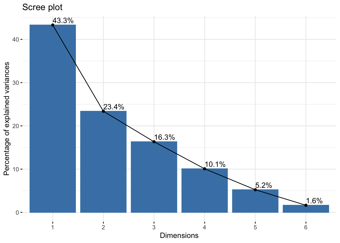
# This plot visualizes both the principal components and the original variables.
# Longer arrows indicate greater contribution
fviz_pca_var(pcaRes,
             # colour by contribution
             col.var = "contrib",
             gradient.cols = "Paired",
             repel = T,
             xlab = "Principal Component 1",
             ylab = "Principal Component 2") + ## takes ggplot arguments
  theme(plot.title = element_text(hjust = 0.5, face = "bold"),
        plot.subtitle = element_text(hjust = 0.5))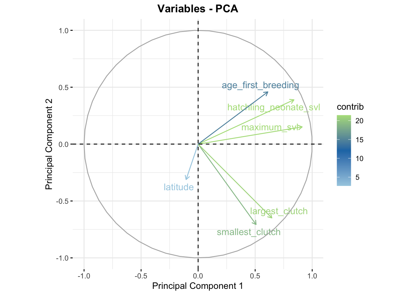
# Next step would be to extract the components to use in an analysis down the road (covered in later modules)

# From here, keep the variables you are interested in exploring for your analysis.
# But beware! Imputation prep is next, and it's not so forgiving!
dfTraits <- dfTraits %>%
  select(family, genus, species, latitude, insular_endemic, maximum_svl,
         hatchling_neonate_svl, activity_time, diet, foraging_mode,
         reproductive_mode, largest_clutch, age_first_breeding,
         iucn_redlist_assessment)

# Write dataset to file for next module.
write.csv(dfTraits, "dfTraits.csv", row.names = F)
Lab Completed!
Congratulations! You have completed Lab 1!