Module 4: Modeling Part 2
Lab
Classification
In this example we’ll be looking at the Pima Indians Diabetes Database collected by the National Institute of Diabetes and Digestive and Kidney Diseases. The dataset contain 768 observations on 9 variables related to the onset of diabetes in women.
Exploratory Data Analysis
diabetes.pc <- diabetes.data  %>%
  mutate(across(c(where(is.numeric)), ~(.x-mean(.x))/sd(.x))) %>%
  dplyr::select(where(is.numeric)) %>%
  cor()

diabetes.pc %>%
  as.data.frame() %>%
  rownames_to_column(var = "Variable_1") %>%
  pivot_longer(cols = -Variable_1, names_to = "Variable_2", values_to = "Correlation") %>%
  ggplot(., aes(x = Variable_1, y = Variable_2, fill = Correlation)) +
  geom_tile() +
  scale_fill_gradient2(low = "blue", high = "red", mid = "white",
                       midpoint = 0, limit = c(-1, 1), space = "Lab",
                       name = "Correlation") +
  theme_minimal() +
  theme(axis.text.x = element_text(angle = 45, vjust = 1, hjust = 1)) +
  coord_fixed() +
  labs(title = "Correlation Matrix of Diabetes Dataset",
       x = "",
       y = "")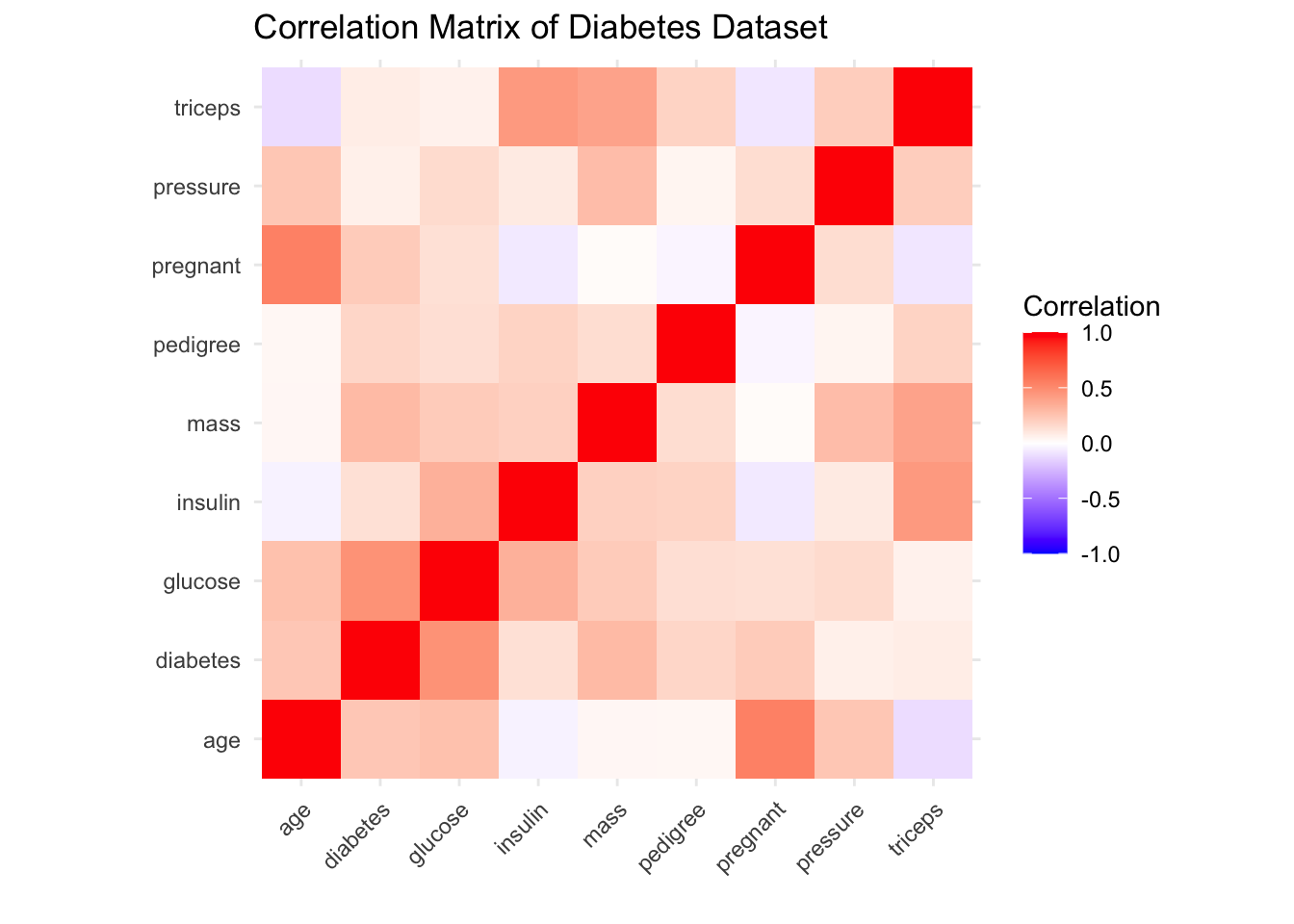
Create Training and Testing Sets
# Split training data into explanatory and response variables
Training.dat <- diabetes.data %>%
  slice_sample(prop = 0.75)

Train.X <- Training.dat %>%
  dplyr::select(-diabetes) %>%
  as.matrix()

Train.Y <- Training.dat %>%
  dplyr::select(diabetes) %>%
  as.matrix()

# Do the same for the testing data
Testing.dat <- diabetes.data %>%
  anti_join(., Training.dat)
## Joining with `by = join_by(pregnant, glucose, pressure, triceps,
## insulin, mass, pedigree, age, diabetes)`Fit a Logistic Regression Model
# Fit a Logistic Regression model
logistic.mod <- glm(diabetes ~ ., data = Training.dat, family = "binomial")

# Predict on training and testing sets
logistic.train <- predict(logistic.mod, newdata = Training.dat, type = "response")
logistic.test <- predict(logistic.mod, newdata = Testing.dat, type = "response")

# Calculate AUC for Logistic Regression
logistic.train.auc <- roc(c(Train.Y), c(logistic.train))
## Setting levels: control = 0, case = 1## Setting direction: controls < cases##
## Call:
## roc.default(response = c(Train.Y), predictor = c(logistic.train))
##
## Data: c(logistic.train) in 375 controls (c(Train.Y) 0) < 201 cases (c(Train.Y) 1).
## Area under the curve: 0.8412## Setting levels: control = 0, case = 1
## Setting direction: controls < cases##
## Call:
## roc.default(response = c(Test.Y), predictor = c(logistic.test))
##
## Data: c(logistic.test) in 125 controls (c(Test.Y) 0) < 67 cases (c(Test.Y) 1).
## Area under the curve: 0.8326Fit an Elastic Net Model
First, you need to identify an optimal lambda value.
Using cross validation for this helps to identify a lambda value which generalizes well as the best one should perform well across all folds.
# Need to conduct cross validation for a more robust estimate or the optimal lambda
foldid <- sample(rep(1:5, length.out = nrow(Training.dat)))

EN.cv.results <- cv.glmnet(Train.X, Train.Y, type.measure="deviance", family="binomial", foldid=foldid, alpha=0.5)

## plot results of 5-fold CV
plot(EN.cv.results)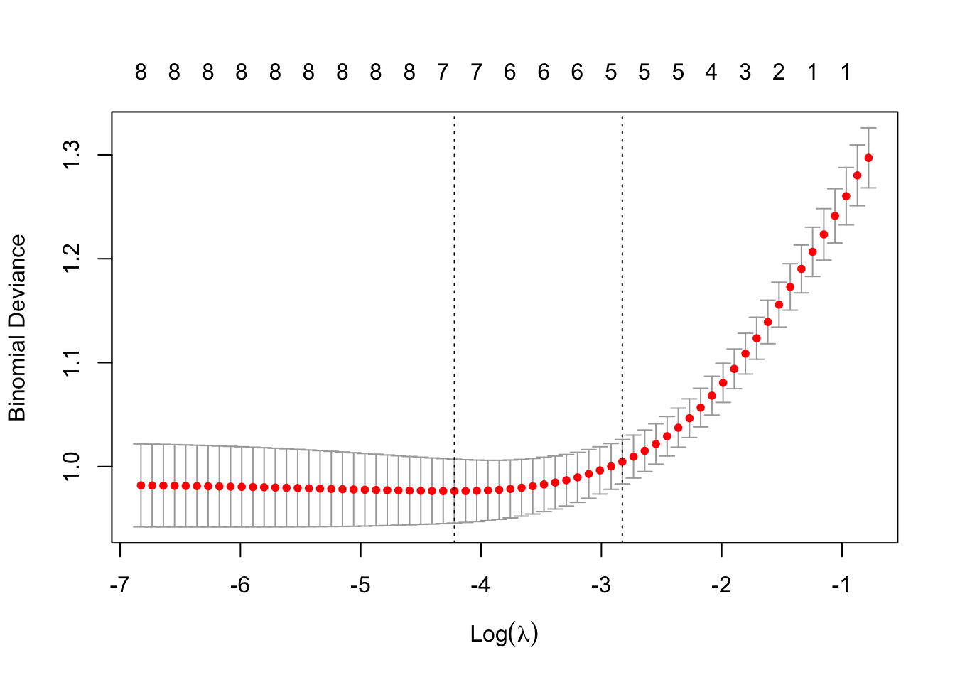
From the deviance-lambda value plot, we see that some amount of regularization is beneficial to model performance, but larger lambda values lead to poor model performance.
Now using the optimal lambda, fit the EN model.
EN.mod <- glmnet(Train.X, Train.Y, type.measure="deviance", family="binomial", lambda = EN.cv.results$lambda.min, alpha=0.5)

## Assess the model performance on the training and testing sets
EN.train <- predict(EN.mod, newx = Train.X, type = "response", s=EN.cv.results$lambda.1se)
EN.test <- predict(EN.mod, newx = Test.X, type = "response", s=EN.cv.results$lambda.1se)

## Calculate the auc for each model
EN.train.auc <- roc(c(Train.Y), c(EN.train))
## Setting levels: control = 0, case = 1## Setting direction: controls < cases## Setting levels: control = 0, case = 1
## Setting direction: controls < cases## Identify and capture the best index for each model
train.snsp <- cbind(EN.train.auc$sensitivities, EN.train.auc$specificities)
train.snsp.best <- which.max(apply(train.snsp, MARGIN = 1 , FUN = min))
## For the testing set
test.snsp <- cbind(EN.test.auc$sensitivities, EN.test.auc$specificities)
test.snsp.best <- which.max(apply(test.snsp, MARGIN = 1 , FUN = min))
## Calculate thresholds scores
EN.train.auc.threshold <- EN.train.auc$thresholds[train.snsp.best]
EN.test.auc.threshold <- EN.test.auc$thresholds[test.snsp.best]
# Extract the coefficients for the chosen lambda
coefficients <- coef(EN.mod, s = 'lambda.min')
# Count the number of non-zero coefficients
num_coefficients <- apply(coefficients != 0, 2, sum)
## join results into a dataframe to return
test.Results <- tibble(
lambda = EN.cv.results$lambda.min,
train_AUC = as.double(EN.train.auc$auc),
test_AUC = as.double(EN.test.auc$auc),
NumCoefficients = num_coefficients
)
test.Results## # A tibble: 1 × 4
## lambda train_AUC test_AUC NumCoefficients
## <dbl> <dbl> <dbl> <int>
## 1 0.0147 0.841 0.829 8Dataset Overview
The GlobalPatterns dataset includes:
- Operational Taxonomic Units (OTUs): OTUs are groups of related organisms. The OTU table records the abundance of each OTU in different samples
- Sample Metadata: This includes information about each sample, such as its source (e.g., soil, freshwater, human gut), which helps us to interpret the clustering results
- Phylogenetic Tree: This tree represents the evolutionary relationships among OTUs
- Taxonomy Data: This provides detailed taxonomic classification (e.g., genus, species) for each OTU
We can use these data to cluster samples based on their microbial community composition, allowing us to explore similarities and differences across environmental samples.
Clustering
Read in Data
# Load example microbiome dataset from phyloseq
data(GlobalPatterns)
microbiome.data <- GlobalPatterns

# Set seed for reproducibility
set.seed(123)
We need to extract the necessary data for the analysis from the data source. We’ll also take a look at the structure of the data.
# Extract the Operational Taxonomic Units (OTU) table and sample data
OTU.data <- otu_table(microbiome.data) %>%
  as.data.frame()
Sample.data <- sample_data(microbiome.data)
Looking at the structure of the OTU data, we can see that the range of values for the variables are quite large and so we’ll need to normalize the data.
##       CL3                CC1                SV1             M31Fcsw
##  Min.   :    0.00   Min.   :    0.00   Min.   :    0.0   Min.   :     0.0
##  1st Qu.:    0.00   1st Qu.:    0.00   1st Qu.:    0.0   1st Qu.:     0.0
##  Median :    0.00   Median :    0.00   Median :    0.0   Median :     0.0
##  Mean   :   44.97   Mean   :   59.09   Mean   :   36.3   Mean   :    80.3
##  3rd Qu.:    3.00   3rd Qu.:    4.00   3rd Qu.:    1.0   3rd Qu.:     0.0
##  Max.   :33783.00   Max.   :36632.00   Max.   :11788.0   Max.   :354695.0
##     M11Fcsw            M31Plmr             M11Plmr            F21Plmr
##  Min.   :     0.0   Min.   :     0.00   Min.   :    0.00   Min.   :    0.000
##  1st Qu.:     0.0   1st Qu.:     0.00   1st Qu.:    0.00   1st Qu.:    0.000
##  Median :     0.0   Median :     0.00   Median :    0.00   Median :    0.000
##  Mean   :   108.1   Mean   :    37.41   Mean   :   22.58   Mean   :    9.695
##  3rd Qu.:     0.0   3rd Qu.:     0.00   3rd Qu.:    0.00   3rd Qu.:    0.000
##  Max.   :452219.0   Max.   :160536.00   Max.   :84880.00   Max.   :14859.000
##     M31Tong            M11Tong             LMEpi24M           SLEpi20M
##  Min.   :     0.0   Min.   :    0.000   Min.   :     0.0   Min.   :     0.0
##  1st Qu.:     0.0   1st Qu.:    0.000   1st Qu.:     0.0   1st Qu.:     0.0
##  Median :     0.0   Median :    0.000   Median :     0.0   Median :     0.0
##  Mean   :   104.1   Mean   :    5.214   Mean   :   110.2   Mean   :    63.3
##  3rd Qu.:     0.0   3rd Qu.:    0.000   3rd Qu.:     0.0   3rd Qu.:     0.0
##  Max.   :540850.0   Max.   :18746.000   Max.   :914209.0   Max.   :323914.0
##      AQC1cm             AQC4cm              AQC7cm              NP2
##  Min.   :     0.0   Min.   :      0.0   Min.   :     0.0   Min.   :    0.00
##  1st Qu.:     0.0   1st Qu.:      0.0   1st Qu.:     0.0   1st Qu.:    0.00
##  Median :     0.0   Median :      0.0   Median :     0.0   Median :    0.00
##  Mean   :    60.8   Mean   :    122.7   Mean   :    88.4   Mean   :   27.25
##  3rd Qu.:     1.0   3rd Qu.:      2.0   3rd Qu.:     1.0   3rd Qu.:    0.00
##  Max.   :554198.0   Max.   :1177685.0   Max.   :711043.0   Max.   :87667.00
##       NP3                 NP5               TRRsed1            TRRsed2
##  Min.   :     0.00   Min.   :     0.00   Min.   :   0.000   Min.   :    0.00
##  1st Qu.:     0.00   1st Qu.:     0.00   1st Qu.:   0.000   1st Qu.:    0.00
##  Median :     0.00   Median :     0.00   Median :   0.000   Median :    0.00
##  Mean   :    76.97   Mean   :    86.01   Mean   :   3.054   Mean   :   25.66
##  3rd Qu.:     0.00   3rd Qu.:     0.00   3rd Qu.:   0.000   3rd Qu.:    1.00
##  Max.   :148400.00   Max.   :161687.00   Max.   :3177.000   Max.   :59245.00
##     TRRsed3              TS28               TS29               Even1
##  Min.   :    0.00   Min.   :    0.00   Min.   :     0.00   Min.   :     0.00
##  1st Qu.:    0.00   1st Qu.:    0.00   1st Qu.:     0.00   1st Qu.:     0.00
##  Median :    0.00   Median :    0.00   Median :     0.00   Median :     0.00
##  Mean   :   14.56   Mean   :   48.79   Mean   :    63.02   Mean   :    63.29
##  3rd Qu.:    0.00   3rd Qu.:    0.00   3rd Qu.:     0.00   3rd Qu.:     0.00
##  Max.   :27172.00   Max.   :92915.00   Max.   :251215.00   Max.   :141771.00
##      Even2               Even3
##  Min.   :     0.00   Min.   :     0.00
##  1st Qu.:     0.00   1st Qu.:     0.00
##  Median :     0.00   Median :     0.00
##  Mean   :    50.53   Mean   :    56.11
##  3rd Qu.:     0.00   3rd Qu.:     0.00
##  Max.   :114624.00   Max.   :124394.00
After normalizing the data the ranges are much more consistent.
##       CL3                CC1                SV1             M31Fcsw
##  Min.   :-0.09916   Min.   :-0.10482   Min.   :-0.1193   Min.   : -0.02682
##  1st Qu.:-0.09916   1st Qu.:-0.10482   1st Qu.:-0.1193   1st Qu.: -0.02682
##  Median :-0.09916   Median :-0.10482   Median :-0.1193   Median : -0.02682
##  Mean   : 0.00000   Mean   : 0.00000   Mean   : 0.0000   Mean   :  0.00000
##  3rd Qu.:-0.09255   3rd Qu.:-0.09772   3rd Qu.:-0.1160   3rd Qu.: -0.02682
##  Max.   :74.40189   Max.   :64.87727   Max.   :38.6148   Max.   :118.40433
##     M11Fcsw             M31Plmr             M11Plmr            F21Plmr
##  Min.   : -0.02402   Min.   : -0.02896   Min.   : -0.0329   Min.   :-0.04842
##  1st Qu.: -0.02402   1st Qu.: -0.02896   1st Qu.: -0.0329   1st Qu.:-0.04842
##  Median : -0.02402   Median : -0.02896   Median : -0.0329   Median :-0.04842
##  Mean   :  0.00000   Mean   :  0.00000   Mean   :  0.0000   Mean   : 0.00000
##  3rd Qu.: -0.02402   3rd Qu.: -0.02896   3rd Qu.: -0.0329   3rd Qu.:-0.04842
##  Max.   :100.48741   Max.   :124.24329   Max.   :123.6427   Max.   :74.16059
##     M31Tong             M11Tong            LMEpi24M            SLEpi20M
##  Min.   : -0.01946   Min.   : -0.0285   Min.   : -0.01623   Min.   : -0.02369
##  1st Qu.: -0.01946   1st Qu.: -0.0285   1st Qu.: -0.01623   1st Qu.: -0.02369
##  Median : -0.01946   Median : -0.0285   Median : -0.01623   Median : -0.02369
##  Mean   :  0.00000   Mean   :  0.0000   Mean   :  0.00000   Mean   :  0.00000
##  3rd Qu.: -0.01946   3rd Qu.: -0.0285   3rd Qu.: -0.01623   3rd Qu.: -0.02369
##  Max.   :101.08524   Max.   :102.4517   Max.   :134.60323   Max.   :121.10293
##      AQC1cm              AQC4cm              AQC7cm
##  Min.   : -0.01488   Min.   : -0.01414   Min.   : -0.01691
##  1st Qu.: -0.01488   1st Qu.: -0.01414   1st Qu.: -0.01691
##  Median : -0.01488   Median : -0.01414   Median : -0.01691
##  Mean   :  0.00000   Mean   :  0.00000   Mean   :  0.00000
##  3rd Qu.: -0.01463   3rd Qu.: -0.01391   3rd Qu.: -0.01672
##  Max.   :135.67447   Max.   :135.76022   Max.   :135.93943
##       NP2                 NP3              NP5              TRRsed1
##  Min.   : -0.03338   Min.   :-0.043   Min.   :-0.04556   Min.   :-0.08325
##  1st Qu.: -0.03338   1st Qu.:-0.043   1st Qu.:-0.04556   1st Qu.:-0.08325
##  Median : -0.03338   Median :-0.043   Median :-0.04556   Median :-0.08325
##  Mean   :  0.00000   Mean   : 0.000   Mean   : 0.00000   Mean   : 0.00000
##  3rd Qu.: -0.03338   3rd Qu.:-0.043   3rd Qu.:-0.04556   3rd Qu.:-0.08325
##  Max.   :107.33978   Max.   :82.863   Max.   :85.59311   Max.   :86.51186
##     TRRsed2            TRRsed3              TS28               TS29
##  Min.   :-0.03810   Min.   :-0.05323   Min.   :-0.03868   Min.   : -0.02521
##  1st Qu.:-0.03810   1st Qu.:-0.05323   1st Qu.:-0.03868   1st Qu.: -0.02521
##  Median :-0.03810   Median :-0.05323   Median :-0.03868   Median : -0.02521
##  Mean   : 0.00000   Mean   : 0.00000   Mean   : 0.00000   Mean   :  0.00000
##  3rd Qu.:-0.03661   3rd Qu.:-0.05323   3rd Qu.:-0.03868   3rd Qu.: -0.02521
##  Max.   :87.91653   Max.   :99.31863   Max.   :73.63814   Max.   :100.47936
##      Even1              Even2            Even3
##  Min.   :-0.04048   Min.   :-0.038   Min.   :-0.03995
##  1st Qu.:-0.04048   1st Qu.:-0.038   1st Qu.:-0.03995
##  Median :-0.04048   Median :-0.038   Median :-0.03995
##  Mean   : 0.00000   Mean   : 0.000   Mean   : 0.00000
##  3rd Qu.:-0.04048   3rd Qu.:-0.038   3rd Qu.:-0.03995
## Max. :90.64845 Max. :86.160 Max. :88.52158Looking at the sample data we get an idea of how the experiment was designed and the different sources of the samples.
##    X.SampleID     Primer   Final_Barcode Barcode_truncated_plus_T
##  AQC1cm : 1   ILBC_01: 1   AACGCA : 1    AACTGT : 1
##  AQC4cm : 1   ILBC_02: 1   AACTCG : 1    ACAGGT : 1
##  AQC7cm : 1   ILBC_03: 1   AACTGT : 1    ACAGTT : 1
##  CC1    : 1   ILBC_04: 1   AAGAGA : 1    ACATGT : 1
##  CL3    : 1   ILBC_05: 1   AAGCTG : 1    ACGATT : 1
##  Even1  : 1   ILBC_07: 1   AATCGT : 1    AGCTGT : 1
##  (Other):20   (Other):20   (Other):20    (Other):20
##   Barcode_full_length              SampleType
##  AGAGAGACAGG: 1       Feces             :4
##  AGCCGACTCTG: 1       Freshwater (creek):3
##  ATGAAGCACTG: 1       Mock              :3
##  CAAGCTAGCTG: 1       Ocean             :3
##  CACGTGACATG: 1       Sediment (estuary):3
##  CATCGACGAGT: 1       Skin              :3
##  (Other)    :20       (Other)           :7
##                                    Description
##  Tijuana River Reserve, depth 2          : 2
##  Allequash Creek, 0-1cm depth            : 1
##  Allequash Creek, 3-4 cm depth           : 1
##  Allequash Creek, 6-7 cm depth           : 1
##  Calhoun South Carolina Pine soil, pH 4.9: 1
##  Cedar Creek Minnesota, grassland, pH 6.1: 1
##  (Other)                                 :19
K Means
k <- 3 # Lets use 3 clusters

kmeans.result <- kmeans(OTU.scaled, centers = k, nstart = 10)

as.factor(kmeans.result$cluster)
## CL3 CC1 SV1 M31Fcsw M11Fcsw M31Plmr M11Plmr F21Plmr
## 1 1 1 2 2 1 1 1
## M31Tong M11Tong LMEpi24M SLEpi20M AQC1cm AQC4cm AQC7cm NP2
## 1 1 1 1 3 3 3 1
## NP3 NP5 TRRsed1 TRRsed2 TRRsed3 TS28 TS29 Even1
## 1 1 2 2 2 2 2 2
## Even2 Even3
## 2 2
## Levels: 1 2 3How do we decide how to choose the number of clusters, K? We can calculate the Within-Cluster Sum of Squares (WCSS). A lower WCSS indicates that data points are closer to their cluster centroids, implying more cohesive clusters.
# Calculate WCSS for different numbers of clusters - Max is 25 as we have 26 groups and min is 2 since having only 1 group is not useful.
wcss <- map(2:25, function(k) {
  kmeans(OTU.scaled, centers = k, nstart = 10)$tot.withinss
})

# Plot WCSS against the number of clusters
plot(2:25, wcss, type = "b", pch = 19, frame = FALSE,
     xlab = "Number of Clusters K",
     ylab = "Within-Clusters Sum of Squares",
     main = "Elbow Method for Determining Optimal Number of Clusters")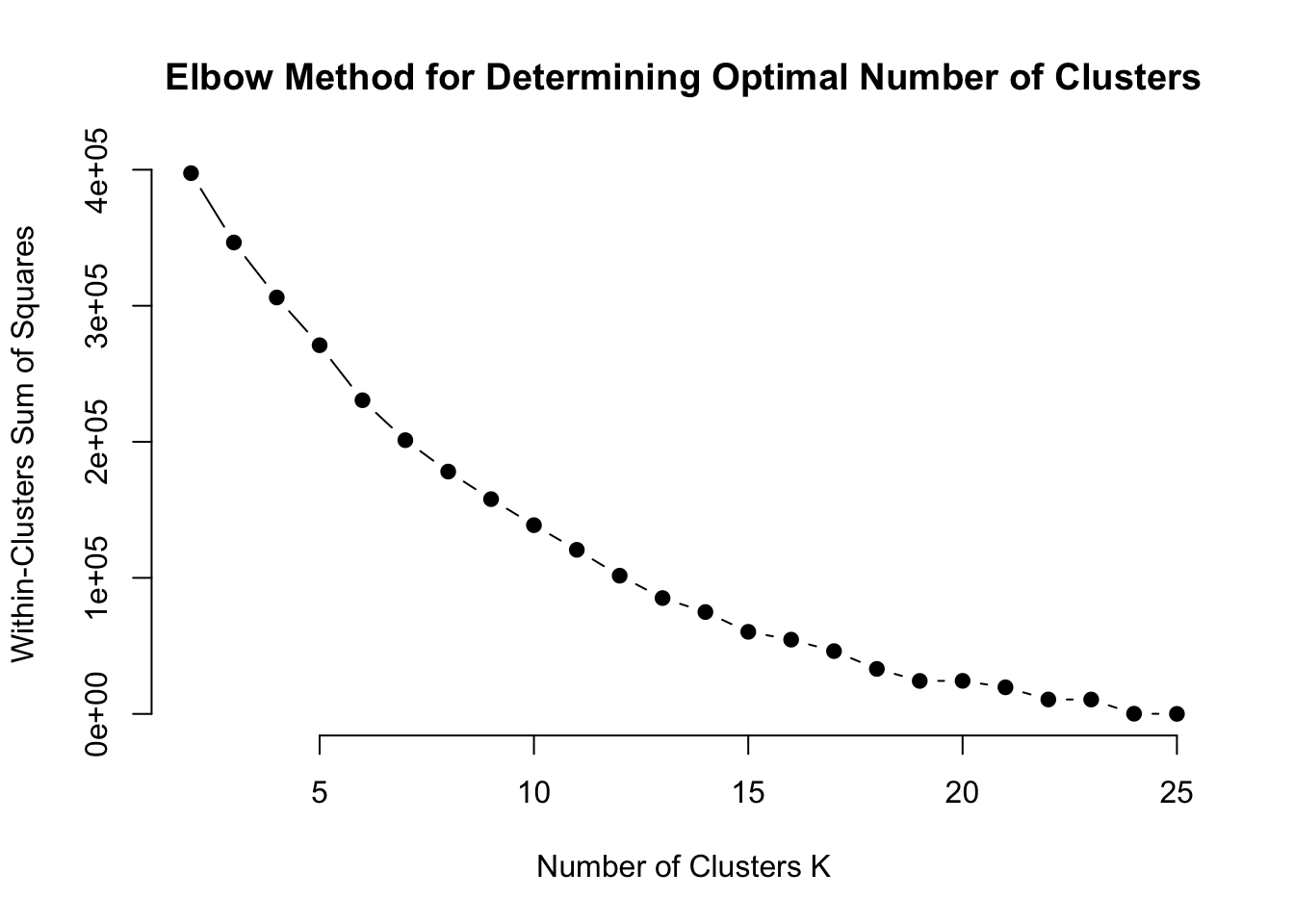
There is no distinct ‘elbow’ on the plot which makes identifying an optimal number of clusters difficult. We’ll refit the model and see how it influences cluster assignments.
Lets set k=15, seems like WCSS doesn’t reduce as quickly after that point.
##      CL3      CC1      SV1  M31Fcsw  M11Fcsw  M31Plmr  M11Plmr  F21Plmr
##        3        1       15        7        7       14       12       14
##  M31Tong  M11Tong LMEpi24M SLEpi20M   AQC1cm   AQC4cm   AQC7cm      NP2
##        5        5        2       11        4        4        4       10
##      NP3      NP5  TRRsed1  TRRsed2  TRRsed3     TS28     TS29    Even1
##        6       10        8        8        8       13       13        9
##    Even2    Even3
##        9        9
## Levels: 1 2 3 4 5 6 7 8 9 10 11 12 13 14 15
These clusters represent groups of samples that are found to be more similar to each other in terms of their OTU abundances.
Let’s evaluate using PCA:
pca_results <- prcomp(OTU.scaled, center = TRUE, scale. = TRUE)
pca_data <- data.frame(pca_results$x, Cluster = as.factor(kmeans.result$cluster))

ggplot(pca_data, aes(PC1, PC2, color = Cluster)) +
  geom_point(size = 2) +
  labs(title = "PCA of OTU Data with 15 K-Means Clusters")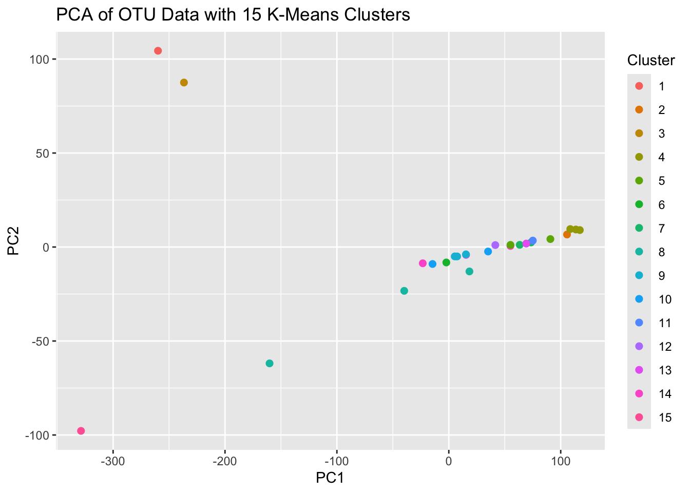
The PCA plot for the 15 cluster K-Means results indicates that we’re probably using too many clusters. Lets reassess with only 4 clusters this time.
kmeans.result2 <- kmeans(OTU.scaled, centers = 4, nstart = 10)

pca_results2 <- prcomp(OTU.scaled, center = TRUE, scale. = TRUE)
pca_data2 <- data.frame(pca_results2$x, Cluster = as.factor(kmeans.result2$cluster))

ggplot(pca_data2, aes(PC1, PC2, color = Cluster)) +
  geom_point(size = 2) +
  labs(title = "PCA of OTU Data with 4 K-Means Clusters")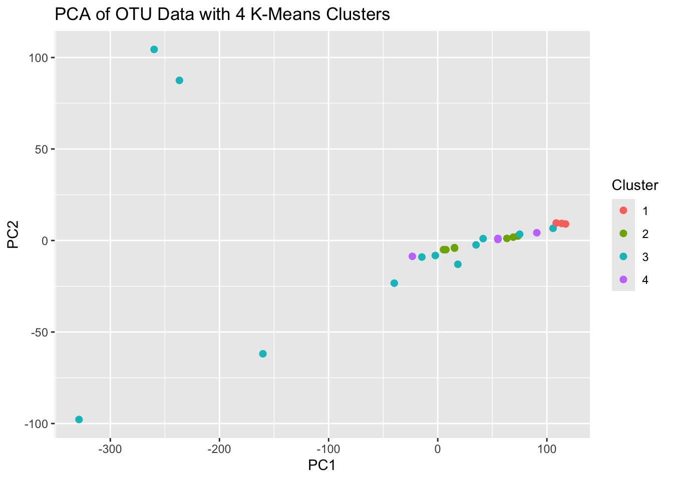
That didn’t cluster the groups as expected,. The proximity of the points on the PCA plot suggests similarity among groups based on the variance captured by the first two PCs, but this may not translate to how the algorithm is determining the number of groups. So, how can we decide what’s best?
- Expert opinion
- Silhouette analysis
- Hierarchical clustering
These are just strategies, they don’t provide a conclusive “optimal” K value.
Let’s explore the silhouette analysis
The Silhouette score measures how similar each point is to its own cluster compared to other clusters. A higher silhouette score suggests better-defined clusters.
silhouette.values <- map(2:10, function(k){
  Kmeans.res <- kmeans(OTU.scaled, centers = k, nstart = 10)
  silhouette.score <- silhouette(Kmeans.res$cluster, dist(OTU.scaled))
  mean(silhouette.score[, 3])  # 3rd column is the silhouette width
})

plot(2:10, silhouette.values, type="b", pch = 19, frame = FALSE,
     xlab="Number of Clusters K",
     ylab="Average Silhouette Width")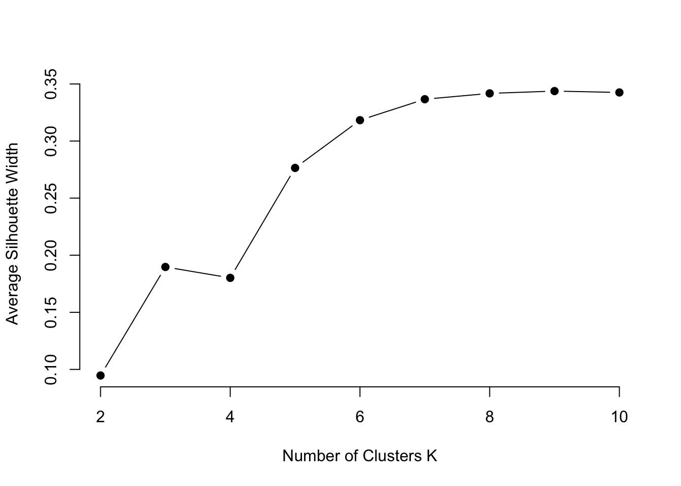
Looks like 6 might be a good choice for our analysis.
Hierarchical Clustering
Hierarchical clustering can help determine where the natural breaks in the data are. We can visually inspect the dendrogram to choose a natural number of clusters.
# Perform hierarchical clustering
hc.res <- hclust(dist(OTU.scaled), method = "complete")

# Plot the dendrogram
plot(hc.res, labels = Sample.data$SampleType, main = "Hierarchical Clustering Dendrogram", xlab = "", sub = "")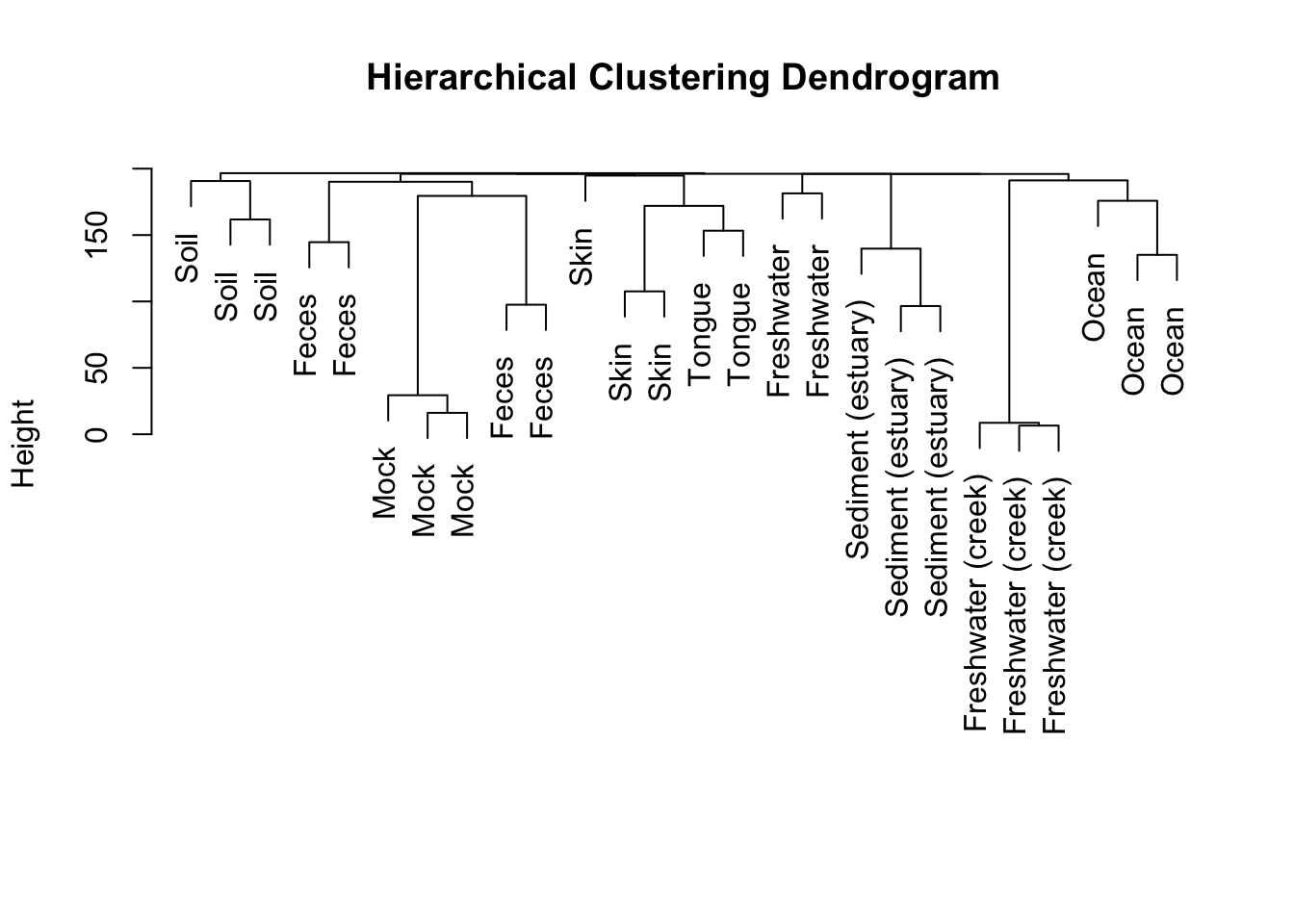
##      CL3      CC1      SV1  M31Fcsw  M11Fcsw  M31Plmr  M11Plmr  F21Plmr
##        1        1        1        2        2        3        4        3
##  M31Tong  M11Tong LMEpi24M SLEpi20M   AQC1cm   AQC4cm   AQC7cm      NP2
##        3        3        5        5        6        6        6        6
##      NP3      NP5  TRRsed1  TRRsed2  TRRsed3     TS28     TS29    Even1
##        6        6        7        7        7        2        2        2
##    Even2    Even3
##        2        2
K-Nearest Neighbours
Typically used for classification, but can be used for clustering.
# Number of neighbors to consider
k <- 7

# Fit KNN model
knn_result <- knn(train = OTU.scaled, test = OTU.scaled, cl = Sample.data$SampleType, k = k)

# Add clustering results to sample data
Sample.data$KNN_Cluster <- knn_result

# Visualize clustering result
table(Sample.data$SampleType, Sample.data$KNN_Cluster)[,1:3]
##
## Feces Freshwater Freshwater (creek)
## Feces 4 0 0
## Freshwater 0 1 1
## Freshwater (creek) 0 0 3
## Mock 3 0 0
## Ocean 0 0 3
## Sediment (estuary) 0 0 0
## Skin 0 0 0
## Soil 0 0 2
## Tongue 0 1 0##
## Mock Sediment (estuary) Skin
## Feces 0 0 0
## Freshwater 0 0 0
## Freshwater (creek) 0 0 0
## Mock 0 0 0
## Ocean 0 0 0
## Sediment (estuary) 2 1 0
## Skin 0 0 3
## Soil 1 0 0
## Tongue 0 0 1The numbers in each cell indicate how many samples of a particular SampleType were assigned to a specific KNN_Cluster. Cluster 1 (first column), contains 4 samples originally labeled as “Feces” and 3 samples originally labeled as “Mock”. This would be considered a mixed cluster as it contains samples from multiple sample types may indicate that those sample types share similar characteristics in terms of OTU data.
Independent Work Section
Load in gene expression data used earlier and clean it to contain only the 1000 most variable genes.
library(tidyverse)
library(TCGAbiolinks)
library(SummarizedExperiment)
library(glmnet)
library(cluster)
You can download the code from the TCGA repository as below, but if that doesn’t work or it takes too long you can use the the next block of code to read in the CSV files instead.
# Lets use the same Gene Expression data as before
query <- GDCquery(project = "TCGA-LAML",
                 data.category = "Transcriptome Profiling",
                 data.type = "Gene Expression Quantification",
                 workflow.type = "STAR - Counts")

GDCdownload(query)
Study.data <- GDCprepare(query)

# Extract the gene expression data
expression.data <- assay(Study.data)

# Transpose the dataset to have samples as rows and genes as columns
expression.data <- t(expression.data)

# Convert to a data frame for easier manipulation
expression.df <- as.data.frame(expression.data)

# Extract the clinical data
clinical.data <- colData(Study.data)
# Or instead load in CSV files of the data - This may also take a minute
# You can do this by providing the path to the data or by using read.csv(file.choose()) instead
expression.df <- read.csv('./datasets/clustering_expression_data.csv') %>% # Use your file path for this data
dplyr::select(-X)
clinical.data <- read.csv('./datasets/clustering_clinical_data.csv') %>% # Use your file path to this data
dplyr::select(barcode, vital_status, age_at_diagnosis) %>%
mutate(vital_status = case_when(vital_status == 'Alive' ~ 1,
vital_status == 'Dead' ~ 0))# Extract the last four digits of the patient identifiers
patient.labels <- substr(clinical.data$patient, nchar(clinical.data$patient) - 3, nchar(clinical.data$patient))
top.genes <- apply(expression.df, 2, var)
top.genes <- sort(top.genes, decreasing = TRUE)
expression.df <- expression.df[, names(top.genes)[1:1000]]
# Standardize the data
expression.df.scaled <- scale(expression.df) %>%
as.data.frame() %>%
dplyr::select(!where(~ sum(is.na(.)) > 0))Conduct K-means clustering as well as hierarchical clustering. How many clusters do you think is optimal?
Create an elbow plot for up to 100 clusters (Or 50 if it takes too long on your computer).
wcss <- map(2:50, function(k) {
  kmeans(expression.df.scaled, centers = k, nstart = 25)$tot.withinss
})

# Plot WCSS against the number of clusters
plot(2:50, wcss, type = "b", pch = 19, frame = FALSE,
     xlab = "Number of Clusters K",
     ylab = "Within-Clusters Sum of Squares",
     main = "Elbow Method for Determining Optimal Number of Clusters")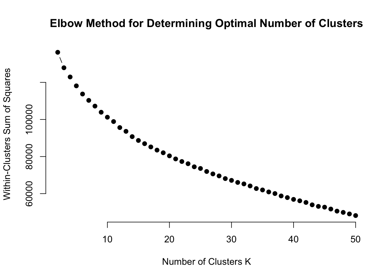
PSelect a number of clusters to use based on the elbow plots and conduct PCA to see if that can further inform your decision.
Kmean.results.20 <- kmeans(expression.df.scaled, centers = 20, nstart = 25)

pca_results <- prcomp(expression.df.scaled, center = TRUE, scale. = TRUE)
pca_data <- data.frame(pca_results$x, Cluster = as.factor(Kmean.results.20$cluster))

ggplot(pca_data, aes(PC1, PC2, color = Cluster)) +
  geom_point(size = 2) +
  labs(title = "PCA of OTU Data with 15 K-Means Clusters")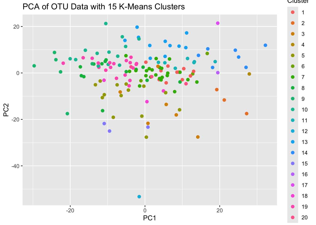
Not very informative.
Conduct a Silhouette analysis up to the number of clusters identified previously.
silhouette.values <- map(2:25, function(k){
  Kmeans.res <- kmeans(expression.df.scaled, centers = k, nstart = 10)
  silhouette.score <- silhouette(Kmeans.res$cluster, dist(expression.df.scaled))
  mean(silhouette.score[, 3])  # 3rd column is the silhouette width
})

plot(2:25, silhouette.values, type="b", pch = 19, frame = FALSE,
     xlab="Number of Clusters K",
     ylab="Average Silhouette Width")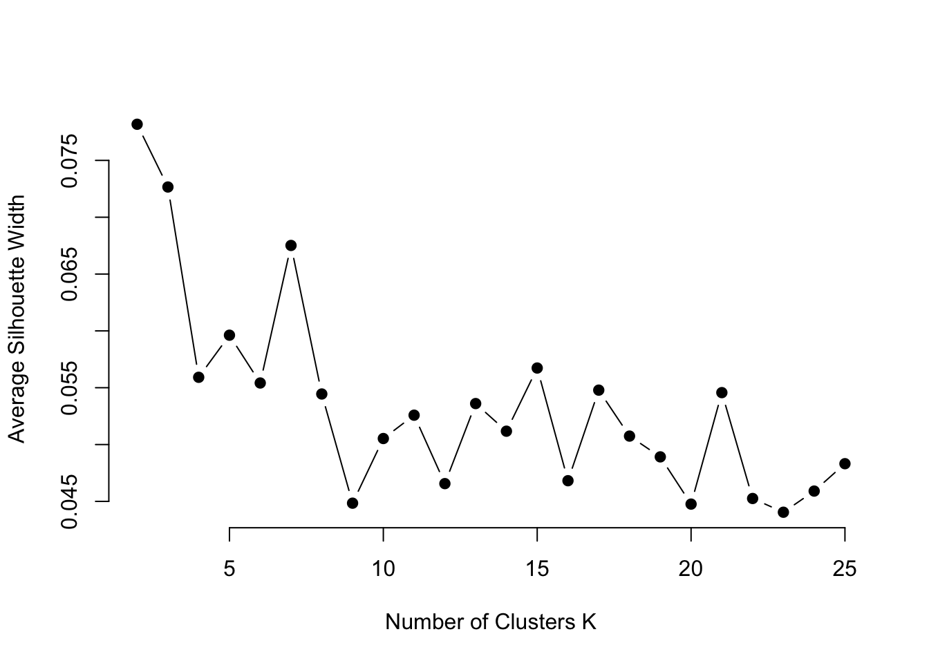
Less than 10 seems to be a good number, lets try 7.
Conduct hierarchical clustering to see if it suggests something different. Use the “patient.labels” object for the labels.
# Perform hierarchical clustering
hc.res <- hclust(dist(expression.df.scaled), method = "complete")

# Plot the dendrogram
plot(hc.res, main = "Hierarchical Clustering Dendrogram", xlab = "", sub = "")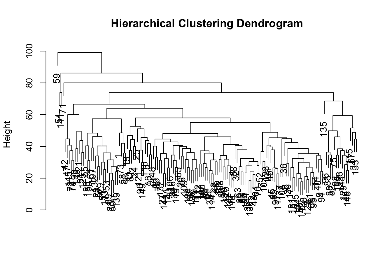
Advanced, join the cluster identification data with the Clinical.data from the classification independent work section. Compare the performance of a logistic regression model fitted to this newly joined dataset against the performance of the EN fit using the Merged.data without cluster IDs. How much information loss is caused by reducing the expression data into clusters vs including it directly into the model?
# Prepare the data
Expression.data <- Study.data %>%
  assay() %>% # Pull out the data
  t() %>% # Transpose the dataset
  as.data.frame() %>%
  rownames_to_column(var = "barcode")

Clinical.data <- colData(Study.data) %>%
  as.data.frame() %>%
  dplyr::select(barcode, vital_status, age_at_diagnosis) %>%
  mutate(vital_status = case_when(vital_status == 'Alive' ~ 1,
                                  vital_status == 'Dead' ~ 0),
         ClusterID = hc.clusters) ## Add cluster ID to the dataset

# Join gene expression data to the clinical outcomes data
Merged.data <- Expression.data[,1:1001] %>% # We're only going to use 1000 of the 60,000 genes available (plus the barcode identifier) for computational efficiency
  left_join(Clinical.data, ., by = 'barcode')
# Split data into training and testing sets
set.seed(123)
Training.data <- Merged.data %>%
slice_sample(prop = 0.8)
Train.X <- Training.data %>%
dplyr::select(-vital_status, -ClusterID) %>%
as.matrix()
Train.Y <- Training.data %>%
dplyr::select(vital_status) %>%
as.matrix()
Testing.data <- Merged.data %>%
anti_join(., Training.data, by = 'barcode')
Test.X <- Testing.data %>%
dplyr::select(-vital_status, -ClusterID) %>%
as.matrix()
Test.Y <- Testing.data %>%
dplyr::select(vital_status) %>%
as.matrix()EN Model
# Perform 5-fold cross-validation for Elastic Net
foldid <- sample(rep(1:5, length.out = nrow(Training.data)))

EN.cv.fit <- cv.glmnet(Train.X, Train.Y, type.measure="deviance", family = "binomial", foldid=foldid, alpha = 0.5)
## Warning in storage.mode(x) <- "double": NAs introduced by coercion
## Warning in storage.mode(x) <- "double": NAs introduced by coercion
## Warning in storage.mode(x) <- "double": NAs introduced by coercion
## Warning in storage.mode(x) <- "double": NAs introduced by coercion
## Warning in storage.mode(x) <- "double": NAs introduced by coercion
## Warning in storage.mode(x) <- "double": NAs introduced by coercion## Warning in cbind2(1, newx) %*% nbeta: NAs introduced by coercion
## Warning in cbind2(1, newx) %*% nbeta: NAs introduced by coercion
## Warning in cbind2(1, newx) %*% nbeta: NAs introduced by coercion
## Warning in cbind2(1, newx) %*% nbeta: NAs introduced by coercion
## Warning in cbind2(1, newx) %*% nbeta: NAs introduced by coercion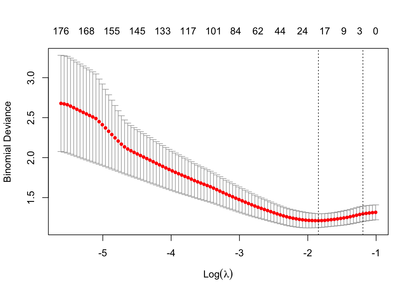
# Fit the Elastic Net model using the optimal lambda from CV
EN.fit <- glmnet(Train.X, Train.Y, family = "binomial", alpha = 0.5, lambda = EN.cv.fit$lambda.min)
## Warning in storage.mode(x) <- "double": NAs introduced by coercion# Predict on training and testing sets
EN.pred.train <- predict(EN.fit, newx = Train.X, type = "response", s = EN.cv.fit$lambda.min)## Warning in cbind2(1, newx) %*% nbeta: NAs introduced by coercion## Warning in cbind2(1, newx) %*% nbeta: NAs introduced by coercion## Setting levels: control = 0, case = 1## Setting direction: controls < cases##
## Call:
## roc.default(response = c(Train.Y), predictor = c(EN.pred.train))
##
## Data: c(EN.pred.train) in 80 controls (c(Train.Y) 0) < 40 cases (c(Train.Y) 1).
## Area under the curve: 0.8937## Setting levels: control = 0, case = 1## Warning in roc.default(Test.Y, EN.pred.test): Deprecated use a matrix as
## predictor. Unexpected results may be produced, please pass a numeric vector.## Warning in roc.default(Test.Y, EN.pred.test): Deprecated use a matrix as
## response. Unexpected results may be produced, please pass a vector or factor.## Setting direction: controls < cases##
## Call:
## roc.default(response = Test.Y, predictor = EN.pred.test)
##
## Data: EN.pred.test in 17 controls (Test.Y 0) < 14 cases (Test.Y 1).
## Area under the curve: 0.6975Logistic Regression Model
# Fit a Logistic Regression model
logistic.mod <- Training.data %>%
  dplyr::select(colnames(Clinical.data), -barcode) %>%
  glm(vital_status ~ ., data = ., family = "binomial")

# Predict on training and testing sets
logistic.train <- Training.data %>%
  dplyr::select(colnames(Clinical.data), -barcode) %>%
  predict(logistic.mod, newdata = ., type = "response")

logistic.test <- Testing.data %>%
  dplyr::select(colnames(Clinical.data), -barcode) %>%
  predict(logistic.mod, newdata = ., type = "response")

# Calculate AUC for Logistic Regression
logistic.train.auc <- roc(c(Train.Y), c(logistic.train))
## Setting levels: control = 0, case = 1## Setting direction: controls < cases##
## Call:
## roc.default(response = c(Train.Y), predictor = c(logistic.train))
##
## Data: c(logistic.train) in 80 controls (c(Train.Y) 0) < 40 cases (c(Train.Y) 1).
## Area under the curve: 0.7059## Setting levels: control = 0, case = 1
## Setting direction: controls < cases##
## Call:
## roc.default(response = c(Test.Y), predictor = c(logistic.test))
##
## Data: c(logistic.test) in 17 controls (c(Test.Y) 0) < 14 cases (c(Test.Y) 1).
## Area under the curve: 0.6639Lab Completed!
Congratulations! You have completed Lab 4!