Informatics on High-Throughput Sequencing Data Module 4 Lab
This work is licensed under a Creative Commons Attribution-ShareAlike 3.0 Unported License. This means that you are able to copy, share and modify the work, as long as the result is distributed under the same license.
CBW HT-seq Module 4 - Single Nucleotide Variant Calling
by Mathieu Bourgey, Ph.D
Table of contents
- Introduction
- Original Setup
- Calling Variants with GATK
- Investigating the SNP calls
- Filter the variants
- Adding functional consequence
- Investigating the functional consequence of variants
- Adding dbSNP annotations
- Overall script
- (Optional) Investigating the trio
- Acknowledgements
Introduction
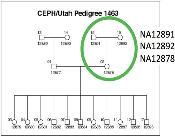
The goal of this practical session is to identify single nucleotide variants (SNVs) in a human genome and to annotate them. In the previous module 3, we have aligned the reads from NA12878 (daughter) in a small region on chromosome 1. We will continue to use the data generated during the Module 3.
NA12878 is the child of the trio while NA12891 and NA12892 are her parents.
For practical reasons we subsampled the reads from the sample because running the whole dataset would take way too much time and resources. We’re going to focus on the reads extracted from a 300 kbp stretch of chromosome 1
| Chromosome | Start | End |
|---|---|---|
| chr1 | 17704860 | 18004860 |
Original Setup
Amazon node
Read these directions for information on how to log in to your assigned Amazon node.
Software requirements
These are all already installed, but here are the original links.
In this session, we will particularly focus on GATK HaplotypeCaller SNV detection tool. The main advantage of HaplotypeCaller is to do the calling using a local de-novo assembly approach. When the program encounters a region showing signs of variation, it discards the existing mapping information and completely reassembles the reads in that region. This allow a better accuracy in regions that are traditionally difficult to call, for example when they contain different types of variants close to each other.
Environment setup
export SOFT_DIR=/usr/local/
export WORK_DIR=~/workspace/HTseq/Module4/
export SNPEFF_JAR=$SOFT_DIR/snpEff/snpEff.jar
export GATK_JAR=$SOFT_DIR/GATK/GenomeAnalysisTK.jar
export BVATOOLS_JAR=$SOFT_DIR/bvatools/bvatools-1.6-full.jar
export REF=$WORK_DIR/reference/


rm -rf $WORK_DIR
mkdir -p $WORK_DIR/variants
cd $WORK_DIR
ln -s ~/CourseData/HT_data/Module4/* .
Data files
The initial structure of your folders should look like this:
ROOT
|-- bam/               # bam file from the previous Module(down sampled)
    `-- NA12878/             # Child sample directory
    `-- NA12891/             # Father sample directory
    `-- NA12892/             # Mother sample directory
`-- reference/               # hg19 reference and indexes
`-- scripts/                 # command lines scripts
`-- saved_results/           # precomputed final files
Cheat sheets
Input files
Let’s look into the NA12878 bam folders
ls bam/NA12878/
Our starting data set consists of 100 bp paired-end Illumina reads from the child (NA12878) that have been aligned to hg19 during one of the previous modules (NA12878.bwa.sort.bam). We also have the same data after duplicate removal, indel realignment and base recalibration (NA12878.bwa.sort.rmdup.realign.bam).
Do you know what are the .bai files? solution
Calling variants with GATK
If you recall from the previous module, we first mapped the reads to hg19 and then we removed duplicate reads and realigned the reads around the indels.
Let’s call SNPs in NA12878 using both the original and the improved bam files:
#NA12878.sort
java -Xmx2g -jar $GATK_JAR -T HaplotypeCaller  -l INFO -R $REF/hg19.fa \
-I bam/NA12878/NA12878.bwa.sort.bam  --variant_index_type LINEAR --variant_index_parameter 128000 -dt none \
-o variants/NA12878.hc.vcf  -L chr1:17704860-18004860

#NA12878.sort.rmdup.realign
java -Xmx2g -jar $GATK_JAR -T HaplotypeCaller -l INFO -R $REF/hg19.fa \
-I bam/NA12878/NA12878.bwa.sort.rmdup.realign.bam  --variant_index_type LINEAR --variant_index_parameter 128000 -dt none \
-o variants/NA12878.rmdup.realign.hc.vcf -L chr1:17704860-18004860
-Xmx2g instructs java to allow up 2 GB of RAM to be used for GATK.
-l INFO specifies the minimum level of logging.
-R specifies which reference sequence to use.
-I specifies the input BAM files.
--variant_index_type LINEAR specifies the indexing strategy to use for VCFs. LINEAR creates a Linear index with bins of equal width, specified by the Bin Width parameter.
--variant_index_parameter 128000 specifies the bin width.
-dt NONE specifies to do not downsample the data.
-L indicates the reference region where SNP calling should take place
Investigating the SNP calls
Use less to take a look at the vcf files:
less -S variants/NA12878.rmdup.realign.hc.vcf
Vcf is a daunting format at first glance, but you can find some basic information about the format here.
Fields vary from caller to caller. Some values are more constant. The ref vs alt alleles, variant quality (QUAL column) and the per-sample genotype (GT) values are almost always there.
How do you figure out what the genotype is for each variant? solution
Do we have any annotation information yet? solution
How many SNPs were found? solution
Did we find the same number of variants using the files before and after duplicate removal and realignment? solution
Looking for differences between the two vcf files
Use the following command to pull out differences between the two files:
diff <(grep ^chr variants/NA12878.hc.vcf | cut -f1-2 | sort) \
<(grep ^chr variants/NA12878.rmdup.realign.hc.vcf | cut -f1-2 | sort)
378d377
< chr1 17927571
Use IGV to investigate the SNPs
The best way to see and understand the differences between the two vcf files will be to look at them in IGV.
If you need, the IGV color codes can be found here: IGV color code by insert size and IGV color code by pair orientation.
Option 1: You can view your files (bam and vcf files) in the IGV browser by using the URL for that file from your Cloud instance. We have a web server running on the Amazon cloud for each instance.
In a browser, like Firefox, type in your server name (cbw#.dyndns.info) and all files under your workspace will be shown there. Find your bam and your vcf files, right click it and ‘copy the link location’.
Next, open IGV and select hg19 as the reference genome as you did in the visualization module.
In IGV, load both the original and the realigned bam files (NA12878.bwa.sort.bam and NA12878.bwa.sort.rmdup.realign.bam) using (File->Load from URL…).
After you have loaded the two bam files, load the two vcf files (NA12878.hc.vcf and NA12878.rmdup.realign.hc.vcf) in the same way.
Option 2: Alternatively, you can download all the NA12878.* files in the current directory to your local computer:
To do this you can use the procedure that was described previously.
After that you need to follow the steps as in Option 1 except that you need to load the files in IGV using (File->Load from File…).
Finally, go to a region on chromsome 1 with reads (chr1:17704860-18004860) and spend some time SNP gazing…
Do the SNPs look believable? solution
Are there any positions that you think should have been called as a SNP, but weren’t? solution
Looking for INDELs
INDELs can be found by looking for rows where the reference base column and the alternate base column are different lengths. It’s slightly more complicated than that since, you’ll also pick up the comma delimited alternate bases.
Here’s an awk expression that almost picks out the INDELs:
grep -v "^#" variants/NA12878.rmdup.realign.hc.vcf \
| awk '{ if(length($4) != length($5)) { print $0 } }' \
| less -S
You can find a slightly more advanced awk script that separates the SNPs from the INDELs here.
Did you find any INDELs? solution
Can you find the largest INDEL? solution
Filter the variants
Typically variant callers will only perform a minimal amount of filtering when presenting variant calls.
To perform more rigorous filtering, another program must be used. In our case, we will use the VariantFiltration tool in GATK.
NOTE: The best practice when using GATK is to use the VariantRecalibrator. In our data set, we had too few variants to accurately use the variant recalibrator and therefore we used the VariantFiltration tool instead.
java -Xmx2g -jar $GATK_JAR -T VariantFiltration \
-R $REF/hg19.fa --variant variants/NA12878.rmdup.realign.hc.vcf -o variants/NA12878.rmdup.realign.hc.filter.vcf --filterExpression "QD < 2.0" \
--filterExpression "FS > 200.0" \
--filterExpression "MQ < 40.0" \
--filterName QDFilter \
--filterName FSFilter \
--filterName MQFilter
-Xmx2g instructs java to allow up 2 GB of RAM to be used for GATK.
-R specifies which reference sequence to use.
--variant specifies the input vcf file.
-o specifies the output vcf file.
--filterExpression defines an expression using the vcf INFO and genotype variables.
--filterName defines what the filter field should display if that filter is true.
What is QD, FS, and MQ? solution
Adding functional consequence
The next step in trying to make sense of the variant calls is to assign functional consequence to each variant.
At the most basic level, this involves using gene annotations to determine if variants are sense, missense, or nonsense.
We typically use SnpEff but many use Annovar and VEP as well.
Let’s run snpEff
java -Xmx2G -jar $SNPEFF_JAR eff \
-c $REF/snpEff_hg19.config -v -no-intergenic \
-i vcf -o vcf hg19 variants/NA12878.rmdup.realign.hc.filter.vcf >  variants/NA12878.rmdup.realign.hc.filter.snpeff.vcf
-Xmx2g instructs java to allow up 4 GB of RAM to be used for snpEff.
-c specifies the path to the snpEff configuration file
-v specifies verbose output.
-no-intergenic specifies that we want to skip functional consequence testing in intergenic regions.
-i and -o specify the input and output file format respectively. In this case, we specify vcf for both.
hg19 specifies that we want to use the hg19 annotation database.
variants/NA12878.rmdup.realign.hc.filter.vcf specifies our input vcf filename
variants/NA12878.rmdup.realign.hc.filter.snpeff.vcf specifies our output vcf filename
Investigating the functional consequence of variants
You can learn more about the meaning of snpEff annotations here.
Use less to look at the new vcf file:
less -S variants/NA12878.rmdup.realign.hc.filter.snpeff.vcf
We can see in the vcf that snpEff added few sections. These are hard to decipher directly from the VCF other tools or scripts, need to be used to make sens of this.
The annotation is presented in the INFO field using the new ANN format. For more information on this field see here. Typically, we have:
ANN=Allele|Annotation|Putative impact|Gene name|Gene ID|Feature type|Feature ID|Transcript biotype|Rank Total|HGVS.c|...
Here’s an example of a typical annotation:
ANN=C|intron_variant|MODIFIER|PADI6|PADI6|transcript|NM_207421.4|Coding|5/16|c.553+80T>C||||||
What does the example annotation actually mean? solution
Next, you should view or download the report generated by snpEff.
Use the procedure described previously to retrieve:
snpEff_summary.html
Next, open the file in any web browser.
Finding impactful variants
One nice feature in snpEff is that it tries to assess the impact of each variant. You can read more about the effect categories here.
How many variants had a high impact? solution
What effect categories were represented in these variants? solution
Open that position in IGV, what do you see? solution
How many variants had a moderate impact? What effect categories were represented in these variants? solution
Adding dbSNP annotations
Go back to looking at your last vcf file:
less -S variants/NA12878.rmdup.realign.hc.filter.snpeff.vcf
What do you see in the third column? solution
The third column in the vcf file is reserved for identifiers. Perhaps the most common identifier is the dbSNP rsID.
Use the following command to generate dbSNP rsIDs for our vcf file:
java -Xmx2g -jar $GATK_JAR -T VariantAnnotator -R $REF/hg19.fa \
--dbsnp $REF/dbSNP_135_chr1.vcf.gz --variant variants/NA12878.rmdup.realign.hc.filter.snpeff.vcf \
-o variants/NA12878.rmdup.realign.hc.filter.snpeff.dbsnp.vcf -L chr1:17704860-18004860
-Xmx2g instructs java to allow up 2 GB of RAM to be used for GATK.
-R specifies which reference sequence to use.
--dbsnp specifies the input dbSNP vcf file. This is used as the source for the annotations.
--variant specifies the input vcf file.
-o specifies the output vcf file.
-L defines which regions we should annotate. In this case, I chose the chromosomes that contain the regions we are investigating.
What percentage of the variants that passed all filters were also in dbSNP? solution
Can you find a variant that passed and wasn’t in dbSNP? solution
(Optional) Investigating the trio
At this point we have aligned and called variants in one individual. However, we actually have FASTQ and BAM files for three family members!
As additional practice, perform the same steps for the other two individuals (her parents): NA12891 and NA12892. Here are some additional things that you might want to look at:
-
If you load up all three realigned BAM files and all three final vcf files into IGV, do the variants look plausible? Use a Punnett square to help evaluate this. i.e. if both parents have a homozygous reference call and the child has a homozygous variant call at that locus, this might indicate a trio conflict. solution
-
Do you find any additional high or moderate impact variants in either of the parents? solution
-
Do all three family members have the same genotype for Rs7538876 and Rs2254135? solution
-
GATK produces even better variant calling results if all three BAM files are specified at the same time (i.e. specifying multiple
-I filenameoptions). Try this and then perform the rest of module 5 on the trio vcf file. Does this seem to improve your variant calling results? Does it seem to reduce the trio conflict rate? solution
Acknowledgements
This module is heavily based on a previous module prepared by Michael Stromberg and Guillaume Bourque.