Module 2
Introduction
Performing Over-Representation Analysis (ORA) with g:Profiler.
The practical lab contains 2 exercises. The first exercise uses g:Profiler to perform gene-set enrichment analysis.
Goal of the exercise 1
Learn how to run g:GOSt Functional profiling from the g:Profiler website and explore the results.
Data
g:Profiler requires a list of genes, one per line, in a text file or spreadsheet, ready to copy and paste into a web page: for this, we use genes with frequent somatic SNVs identified in TCGA exome sequencing data of 3,200 tumors of 12 types. The MuSiC cancer driver mutation detection software was used to find 127 cancer driver genes that displayed higher than expected mutation frequencies in cancer samples (Supplementary Table 1, which is derived from column B of Supplementary Table 4 in Kandoth C. et al.. Genes are ranked in decreasing order of significance (FDR Q value) and mutation frequency (not shown).
Exercise 1 - run g:Profiler
For this exercise, our goal is to run an analysis with g:Profiler. We will copy and paste the list of genes into the g:Profiler web interface, adjust some parameters (e.g selecting the pathway databases), run the query and explore the results.
g:Profiler performs a gene-set enrichment analysis using a hypergeometric test (Fisher’s exact test) with the option to consider the ranking of the genes in the calculation of the enrichment significance (minimum hypergeometric test). The Gene Ontology Biological Process, Reactome and WikiPathways sources are going to be used as pathway databases. The results are displayed as a table or downloadable as an Generic Enrichment Map (GEM) output file.
Before starting this exercise, download the required files:
Right click on link below and select “Save Link As…”.
Place it in the corresponding module directory of your CBW work directory.
We recommend saving all these files in a personal project data folder before starting. We also recommend creating an additional result data folder to save the files generated while performing the protocol.
Step 1 - Launch g:Profiler.
Open the g:Profiler website at g:Profiler in your web browser.
Step 2 - input query
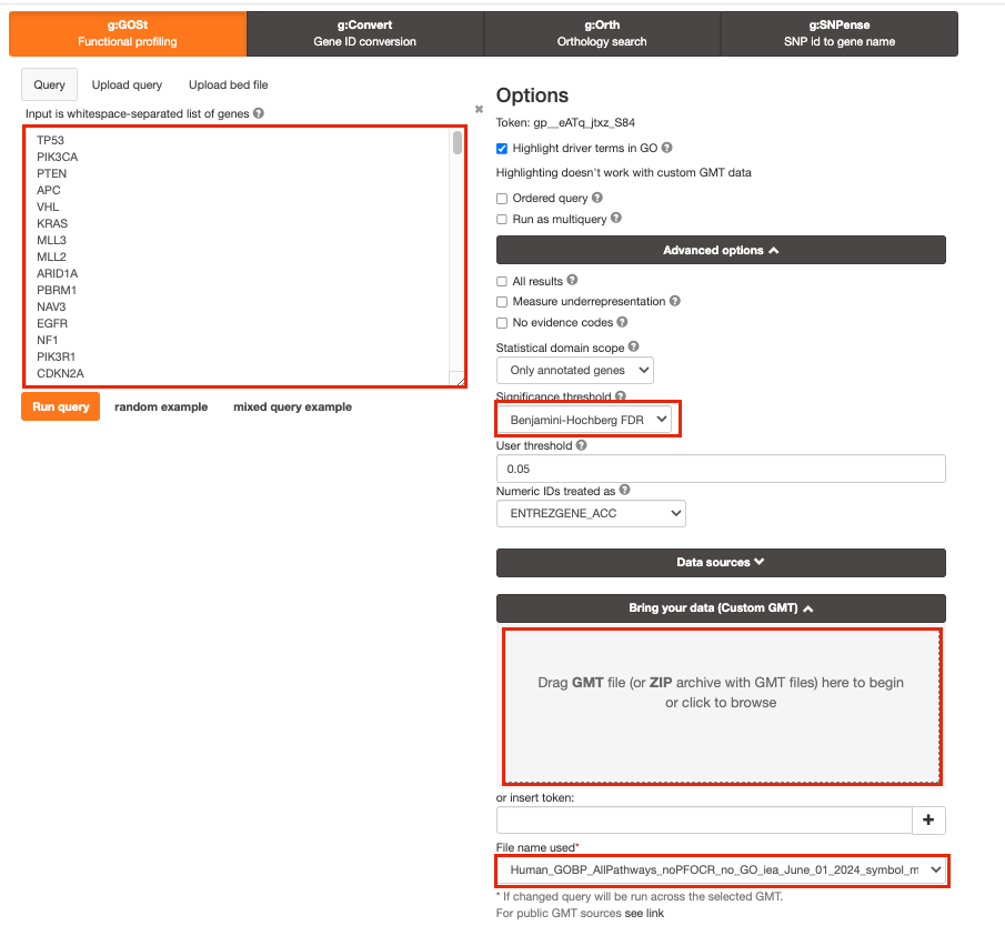
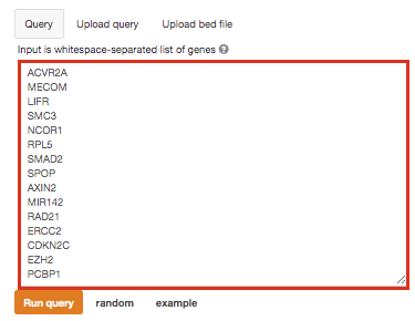
Paste the gene list (Pancancer_genelist.txt) into the Query field in top-left corner of the screen.
Open the file in a simple text editor such as Notepad or Textedit to
copy the list of genes.
Or right click on the file name above and
select Open link in new tab
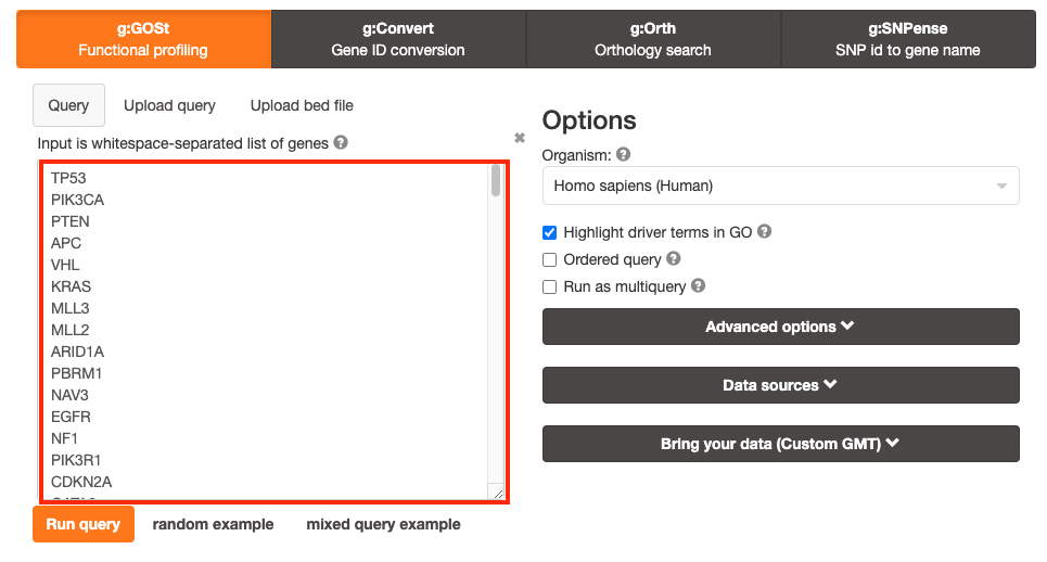
The gene list can be space-separated or one per line.
The
organism for the analysis, Homo sapiens, is selected by default.
The
input list can contain a mix of gene and protein IDs, symbols and
accession numbers.
Duplicated and unrecognized IDs will be removed
automatically, and ambiguous symbols can be refined in an interactive
dialogue after submitting the query.
Highlight driver terms
in GO is a recently (April 2023) added feature that tries to
reduce the number of GO terms returned by g:Profiler and highlight a
non-redundant set of GO terms. For more detailed information on this
feature see here
Step 3 - Adjust parameters.
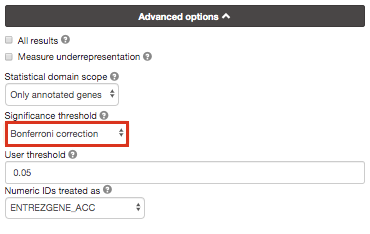
3a. Click on the Advanced options tab (black rectangle) to expand it.
Set Significance threshold to “Benjamini-Hochberg FDR”
User threshold - select 0.05 if you want g:Profiler to return only pathways that are significant (FDR < 0.05).
If g:Profiler does not return any results increase the threshold (0.1, then 1) to check that g:Profiler is running successfully but there are simply no significant results for your query.
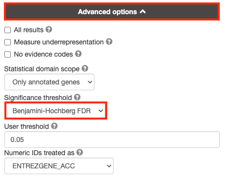
By default, g:Profiler will only return the sets that pass the defined threshold. Often you need the ability to tweak the thresholds in the resulting EM beyond the strict FDR < 0.05 threshold and therefore require all the results. In order to get all the results, even those that don’t pass correction, select All results.
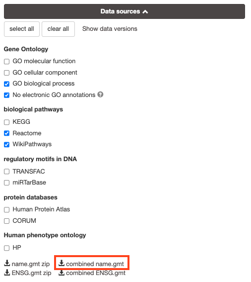
3b. Click on the Data sources tab (black rectangle) to expand it.
- Unselect all gene-set databases by clicking the “clear all” button.
- In the Gene Ontology category, check GO Biological Process and No electronic GO annotations.
- In the biological pathways category, check Reactome and check WikiPathways.
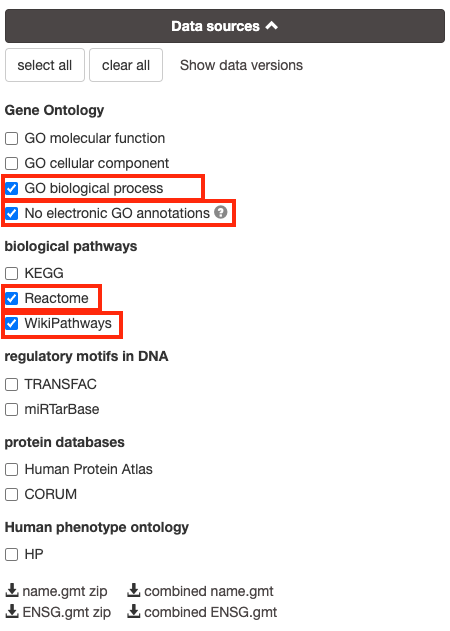
No electronic GO annotations option will discard less reliable GO annotations (inferred from electronic annotations (IEAs)) that are not manually reviewed.
if g:Profiler does not return any results uncheck the No electronic GO annotation option to expand annotations used in the test.
Step 4 - Run query
Click on the Run query button, below the input parameters, to run g:Profiler.
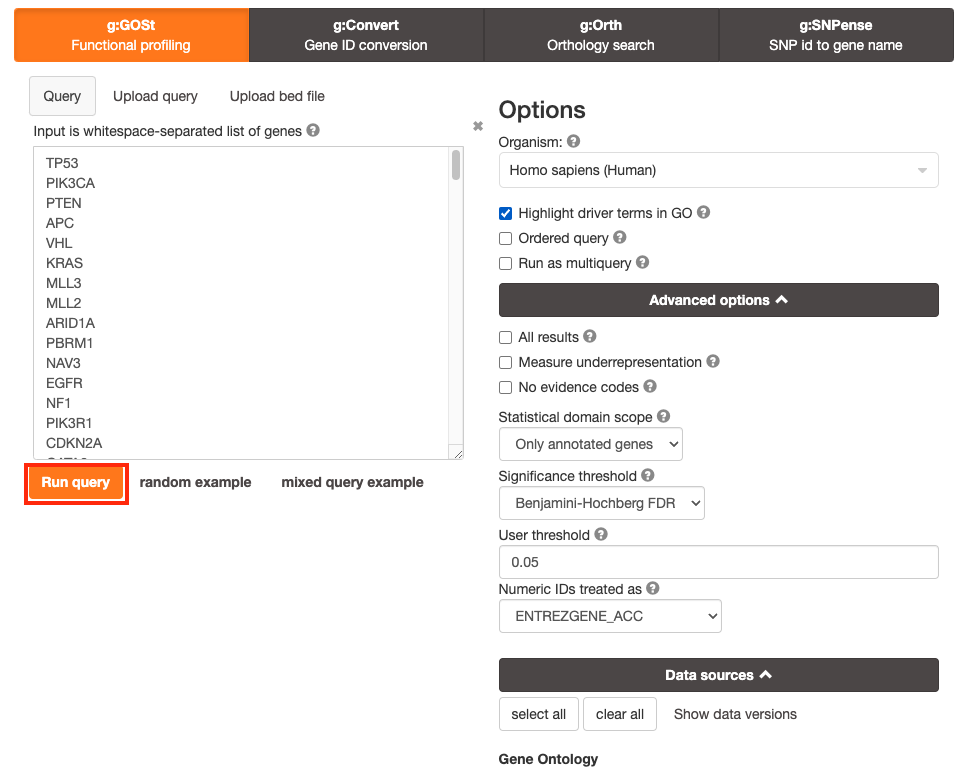
Scroll down page to see results.
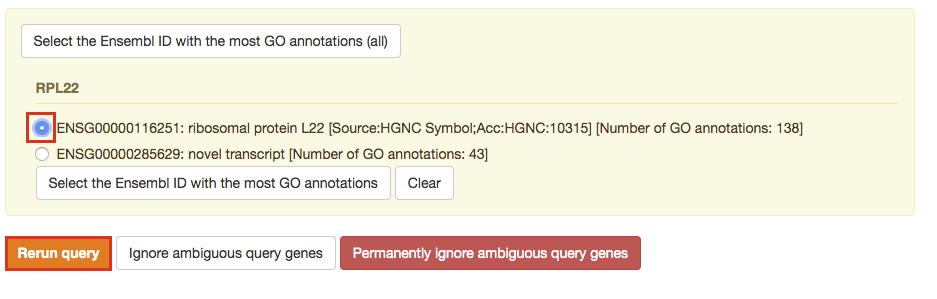
After clicking on Run query button, the analysis completes but if there is the following message (above results) - Select the Ensembl ID with the most GO annotations (all), then do the following. For each ambiguous gene, select its correct mapping. Ambiguous mapping is often caused by multiple Ensembl ids for a given gene and are easy to resolve as a user. Rerun query.
Step 5 - Explore the results.
Step 5a:
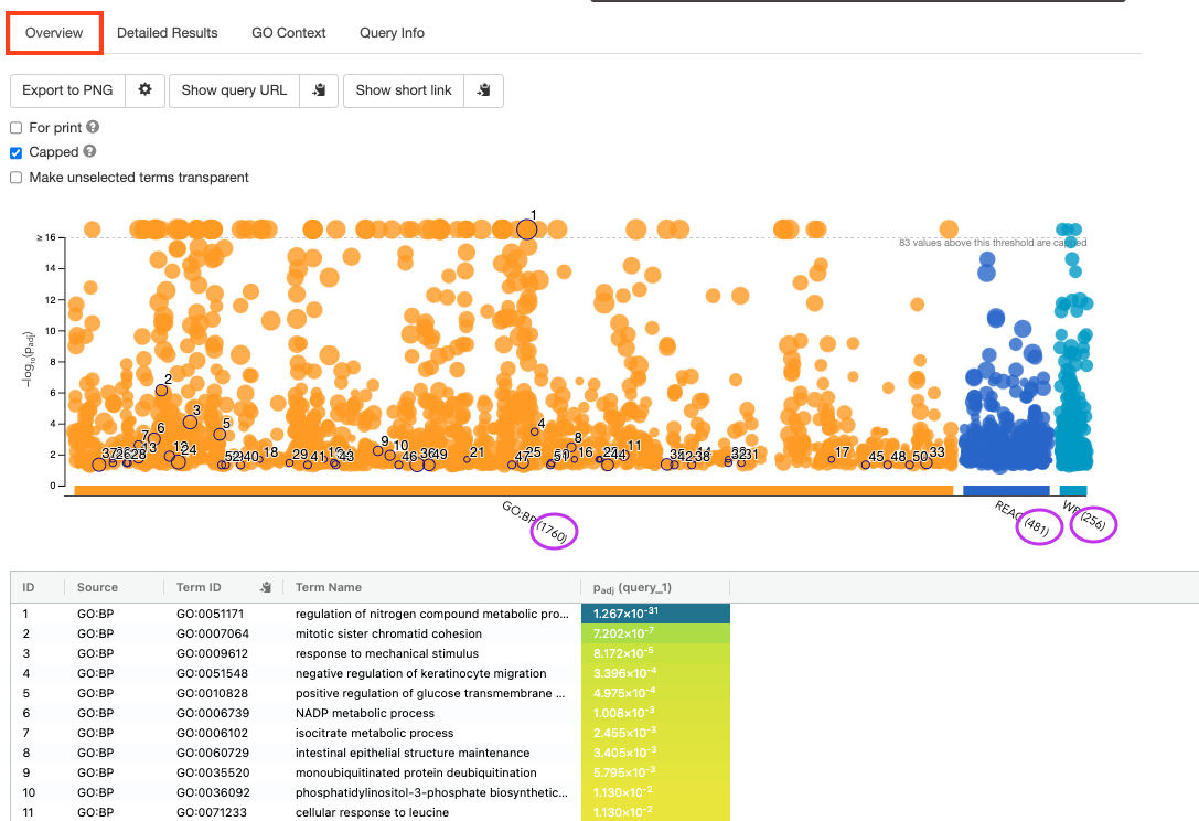
- After the query has run, the results are displayed at the bottom of the page, below the input parameters.
- By default, the “Overview” tab is selected. A global graph displays gene-sets that passed the significance threshold of 0.05 for each of the 3 data sources (shown on x-axis) that we have selected - GO Biological Process(GO:BP) and Reactome(REAC) and WikiPathways(WP). Numbers in parentheses indicate the number of gene-sets that passed the threshold.
Step5b:
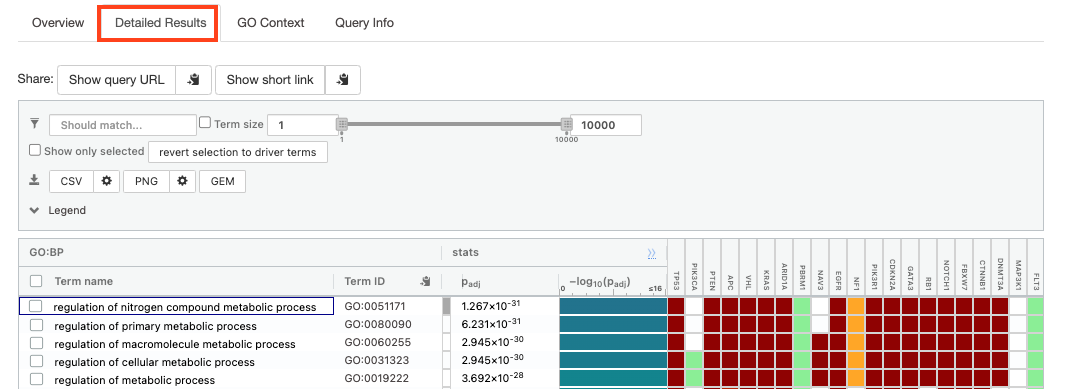
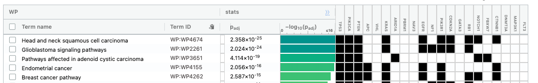
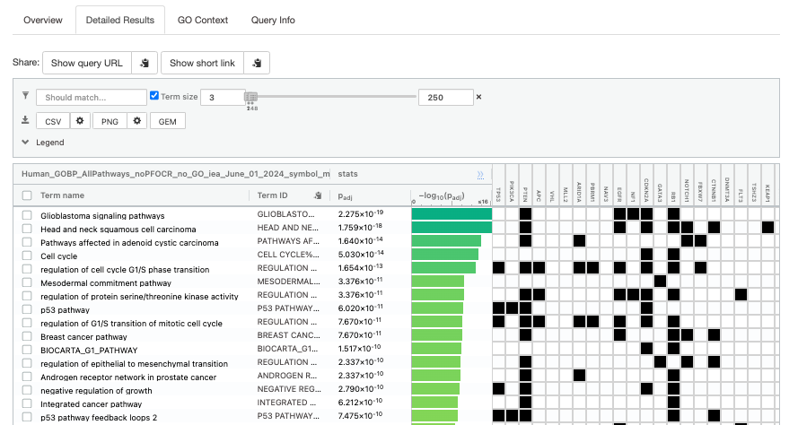
- Click on “Detailed Results” to view the results in more depth. Three tables are displayed, one for each of the data sources selected. (If more than 3 data sources are selected there will be additional tables for each data source). Each row of the table contains:
- Term name - gene-set name
- Term ID - gene-set identifier
- Padj - FDR value
- -log10(Padj) - enrichment score calculated using the formula -log10(padj)
- Variable number of gene columns (One for each gene in the query set) - If the gene is present in the current gene-set its cell is colored. For any data source besides GO, the cell is colored black if the gene is found in the gene-set. For the GO data source cells are colored according to the annotation evidence code. Expand the Legend tab for detailed coloring mapping of GO evidence codes.
The first table displays the gene-sets significantly enriched at FDR 0.05 for the GO:BP database.
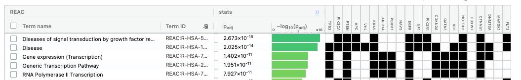
The second table displays the results corresponding to the Reactome database.
The third table displays the results corresponding to the WikiPathways database.
Step 6: Expand the stats tab
Expand the stats tab by clicking on the double arrow located at the right of the tab.
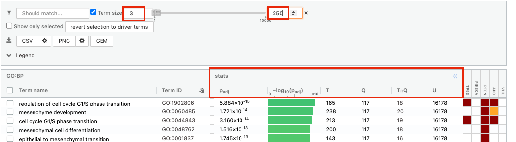
It displays the gene set size (T), the size of our gene list (Q) , the number of genes that overlap between our gene list and the tested gene-set (TnQ) as well as the number of genes in the background (U).
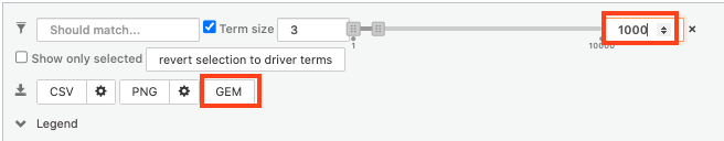
- Above the GO:BP result table, locate the slide bar that enables to select for the minimum and maximum number of genes in the tested gene-sets (Term size).
- Change the maximum Term size from 10000 to 250 and
- Change the minimum Term size from 1 to 3 and
- Observe the results in the detailed stats panel:
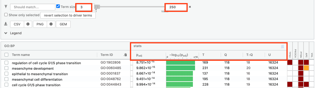
- Without filtering term size, the top terms were GO terms containing more than 4000 or 5000 genes and often terms located high in the GO hierarchy (parent term).
- With filtering the maximum term size to 250, the top list contains pathways with larger interpretative values. However, please note that the adjusted p-values were calculated using all gene-sets without size filtering.
Step 7: Save the results
7a. In the Detailed Results panel, select “GEM” . It will save the results in a text file in the “Generic Enrichment Map” format that we will use to visualize using Cytoscape.
- keep the minimum term size set to 3 (for all the three files we create below)
- set maximum term size to 10000 ( = no filtering by gene-set size) and click on the GEM button. A file is downloaded on your computer. (change the name to gProfiler_hsapiens_lab2_results_GEM_termmin3_max10000.gem.txt)
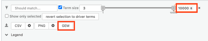
- set maximum term size to 1000 ( = filter by gene-set size) and click on the GEM button. A file is downloaded on your computer. (change the name to gProfiler_hsapiens_lab2_results_GEM_termmin3_max1000.gem.txt)
- select max term size to 250 ( = filter by gene-set size) and click on the GEM button. A file is downloaded on your computer. (change the name to gProfiler_hsapiens_lab2_results_GEM_termmin3_max250.gem.txt)
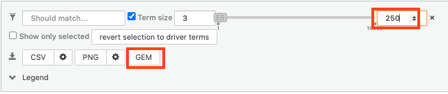
7b: Open the file that you saved using the gene-set threshold of 250 using Microsoft Office Excel or in an equivalent software.
Observe the results included in this file:
- Name of each gene-set
- Description of each gene-set
- Significance of the overlap (pvalue)
- Significance of the overlap (adjusted pvalue/qvalue)
- Phenotype
- Genes included in each gene-set
Which GO:BP term has the best corrected p-value?
Which genes in
our list are included in this term?
Observe that some genes can be
present on several lines (pathways are related when they contain a lof
of genes in common).
The table is formatted for the input into Cytoscape EnrichmentMap. It is called the generic format. The p-value and FDR columns contain identical values because g:Profiler directly outputs the FDR (= corrected p-value) meaning that the p-value column is already the FDR. Phenotype 1 means that each pathway will be represented by red nodes on the enrichment map (presented during next module).
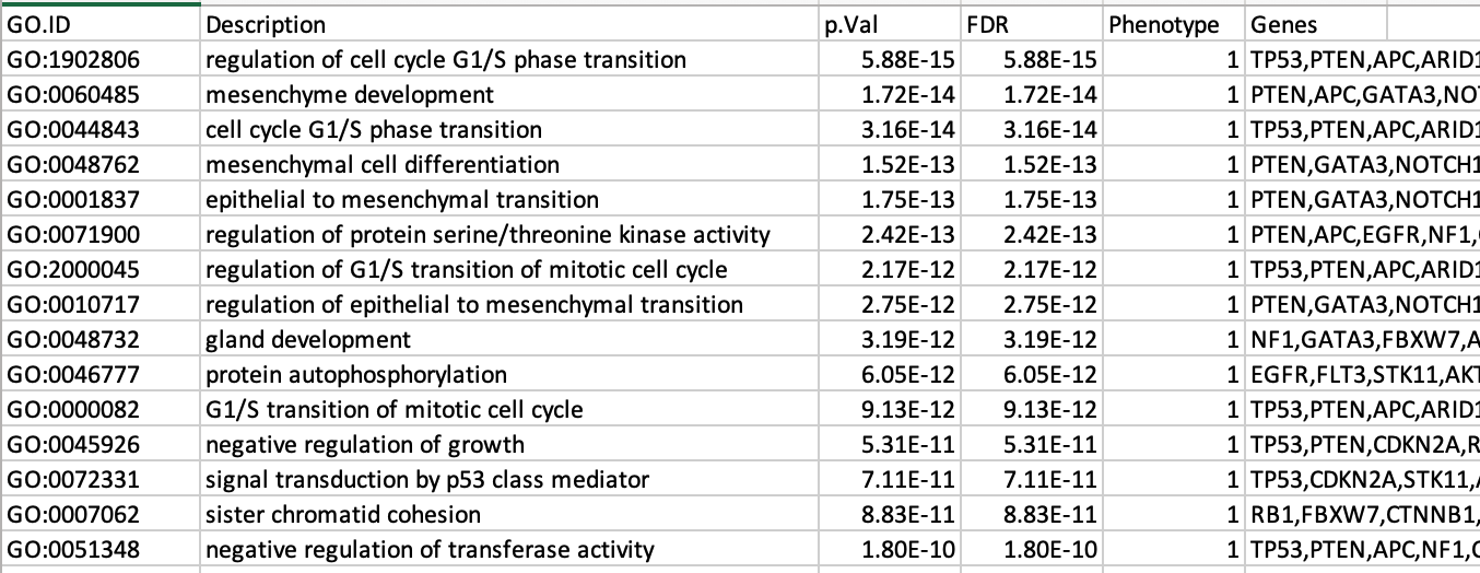
The GO:BP term regulation of cell cycle G1/S phase transition is the most significant gene-set (=the lowest FDR value). Many gene-sets from the top of this list are related to each other and have genes in common.
Step 8 (Optional but recommended)
8a. Download the pathway database files.
- Go to the top of the page and expand the “Data sources” tab. Click on the ‘combined name.gmt’ link located at bottom of this tab. It will download a file named combined name.gmt containing a pathway database gmt file with all the available sources.
8b. concatenate the GO:BP, Reactome and WikiPathways gmt files:
If you want to create a smaller gmt file that doesn’t contain all of the g:profiler datasources you can instead download name.gmt.zip that contains each datasource as its own gmt file. You will need to concatenate the sources you require into one gmt file to use for later.
Option 1: manually if you are not familiar with unix commands
- open a text editor such a Notepad or equivalent
- open hsapiens.GO:BP.name.gmt using the text editor
- open gmt hsapiens.REAC.name.gmt using the text editor
- copy-paste all the rows from REAC file together with all the rows in GO:BP file.
- open gmt hsapiens.WP.name.gmt using the text editor
- copy-paste all the rows from WP file together with all the rows in GO:BP file.
- save the file as hsapiens.pathways.name.gmt .
Option 2: using the cat command if you are familiar with unix commands
- open your terminal window
- cd to the unzipped gprofiler_hsapiens.name folder
- type the following command:
cat hsapiens.GO:BP.name.gmt hsapiens.REAC.name.gmt hsapiens.WP.name.gmt > hsapiens.pathways.name.gmtyou will be using this optional hsapiens.pathways.name.gmt file in Cytoscape EnrichmentMap.
Step 9 (Optional by recommended)
- Get and record the version of g:Profiler used in your analysis. It is important to note in your future publication using your enrichment results the methods and the version of software used for any analysis. g:Profiler is updated on a regular basis so you can not simply come back to the webpage at time of publication and get the version. Also, if you ever want to verify the results that you have and re-run the analysis it is important to use the same version as the initial analysis (or your results might differ). g:Profiler maintains an archive so it is easy to revisit previous versions.
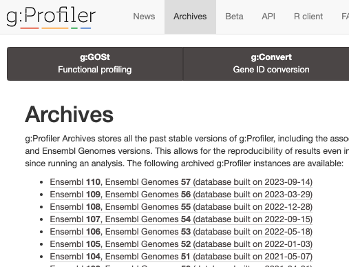
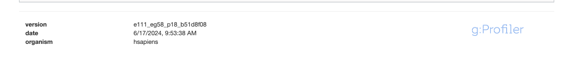
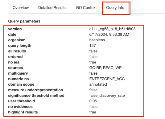
- The g:Profiler version can be found in two places -
- At the bottom of overview tab the version is listed
- Or Click on the Query Info tab to see all the parameters, including the g:Profiler version, used for the analysis
- At the bottom of overview tab the version is listed
Deciphering the version from the listed tag e111_eg58_p18_b51d8f08
:
* e111 - Ensembl version 111
* eg56 - Ensembl genomes version
58
The version info can be recorded anywhere (for example in your lab
notebook) but a convenient place is to embed it in the g:Profiler
geneset file name used for the analysis.
Instead of naming the file
* hsapiens.pathways.name.gmt
Name it
*
hsapiens.pathways_e111_eg58_p18_b51d8f08.name.gmt
Exercise 2: Load and use a custom .gmt file and run the query
For this exercise, our goal is to copy and paste the list of genes into g:Profiler, upload a custom gmt file, adjust some parameters (e.g selecting the pathway databases), run the query and explore the results. Uploading a custom gmt file enables us to use alternate pathway data sources not available in g:Profiler.
We are going to use a gmt file that contains a database of pathway gene sets used for pathway enrichment analysis in the standard GMT format downloaded from http://baderlab.org/GeneSets and updated monthly.
This file contains pathways from eight data sources:
- GO,
- Reactome,
- Panther,
- NetPath,
- NCI,
- MSigDB curated gene sets (C2 collection, excluding Reactome and KEGG),
- MSigDB Hallmark (H collection) and
- HumanCyc.
A GMT file is a text file in which each line represents a gene set for a single pathway. Each line includes a pathway ID, a name and the list of associated genes in a tab-separated format. This file has been filtered to exlclude gene-sets that contained more than 250 genes as these gene-sets are associated with more general terms.
Before starting this exercise, download the required files:
Right click on link below and select “Save Link As…”.
Place it in the corresponding module directory of your CBW work directory.
We recommend saving all these files in a personal project data folder before starting. We also recommend creating an additional result data folder to save the files generated while performing the protocol.
STEPS:
Repeat step 1 to 3a from Exercise 1 (go back to exercise 1 to get detailed instructions) Briefly:
- Step 1:
- Open g:profiler
- Step 2a :
- Copy and paste the gene list in the Query field
- Step 2b: Click on the Advanced options tab (black rectangle) to expand it.
- Set Significance threshold to “Benjamini-Hochberg FDR”.
- Step 3a: Click on the Data sources tab (black rectangle) to expand it.
- Unselect all choices by clicking the “clear all” button.
- Step 4: Click on the Custom GMT tab (black rectangle) to expand it.
- Drag in the box the Baderlab gmt file Baderlab_genesets.gmt.
- Once uploaded successfully, the name of the file is displayed in the “File name used” box.
Step 5: Click on Run query .
Step 6: Explore the detailed results
Step 7: Save the file as GEM (rename file to gProfiler_hsapiens_Baderlab_max250.gem.txt)
- Step 1:
Optional steps
Please follow these optional steps if time permits and/or to explore more g:Profiler parameters.
Here below are 3 optional steps that cover several options offered by g:Profiler:
- test different data sources,
- take the order of the gene list into account,
- use different types of multiple hypothesis correction methods.
Use the same gene list as used in exercise 1 and modify paramters listed above. Observe the results.
Optional 1:
If time permits, play with input parameters, e.g. add TRANSFAC and miRTarBase databases, rerun the query and explore the new results.
Transfac putative transcription factor binding sites
(TFBSs) from TRANSFAC database are retrieved into g:GOSt through a
special prediction pipeline. First, TFBSs are found by matching TRANSFAC
position specific matrices using the program Match on range +/-1kb from
TSS as provided by APPRIS (Annotating principal splice isoforms) via
Ensembl biomart. For genes with multiple primary TSS annotations we
selected one with most TF matches. The matching range for C. elegans, D.
melanogaster and S. cerevisiae is 1kb upstream from ATG (translation
start site). A cut-off value to minimize the number of false positive
matches (provided by TRANSFAC) is then applied to remove spurious
motifs. Remaining matches are split into two inclusive groups based on
the amount of matches, i.e TFBSs that have at least 1 match are
classified as match class 0 and TFBSs that have at least 2 matches per
gene are classified as match class 1.
mirTarBase is a database that holds experimentally
validated information about genes that are targetted by miRNAs. We
include all the organisms that are covered by mirTarBase.
Option 2:
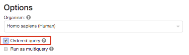
Re-run the g:Profiler using the ordered query checked.
This will run the minimum hypergeometric test. g:Profiler then performs incremental enrichment analysis with increasingly larger numbers of genes starting from the top of the list. When this option is checked, it assumes that the genes were preordered by significance with the most significant gene at the top of the list.
Compare the results between “ordered” and non ordered query.
for this practical lab, the genes were ordered by the number of
mutations found in these genes for all samples.
For example, TP53, a
highly mutated genes is listed at the top.
Option 3 :
Re-run g:Profiler and select g:SCS or Bonferonni as method to correct for multiple hypothesis testing. Do you get any significant results?
you can get detailed information about these methods at https://biit.cs.ut.ee/gprofiler/page/docs in the section Significance threshold.
Bonus - Automation.
Run analysis directly from R for easy integration into existing pipelines.
Instead of using the g:Profiler website g:profiler can be run directly from R or python see g:Profiler document for more info at https://biit.cs.ut.ee/gprofiler/page/r
Follow the step by step instructions on how to run from R here - https://risserlin.github.io/CBW_pathways_workshop_R_notebooks/run-gprofiler-from-r.html
First, make sure your environment is set up correctly by following there instructions - https://risserlin.github.io/CBW_pathways_workshop_R_notebooks/setup.html
Introduction
This practical lab contains one exercise. It uses GSEA to perform a gene-set enrichment analysis.
Data
The data used in this exercise is gene expression (transcriptomics) obtained from high-throughput RNA sequencing of Pancreatic Ductal Adenocarcinoma samples (TCGA-PAAD).
This cohort has been previously stratified into many different set of subtypes PMID:36765128 with the Moffitt Basal vs Classical subtypes compared to demonstrate the GSEA workflow.
How was the data processed?
- Gene expression from the TCGA Pancreatic Ductal Adenocarcinoma RNASeq cohort was downloaded on 2024-06-06 from Genomic Data Commons using the TCGABiolinks R package.
- Differential expression for all genes between the Basal and Classical groups was estimated using edgeR.
- The R code used to generate the data and the rank file used in GSEA is included at the bottom of the document in the Additional information section.
Background
The goal of this lab is to:
- Upload the 2 required files into GSEA,
- Adjust relevant parameters,
- Run GSEA,
- Open and explore the gene-set enrichment results.
The 2 required files are:
- a rank file (.rnk)
- a pathway definition file (.gmt).
Rank File
To generate a rank file (.rnk), a score (-log10(pvalue) * sign(logFC)) was calculated from the edgeR differential expression results. A gene that is significantly differentially expressed (i.e associated with a very small pvalue, close to 0) will be assigned a high score.
The sign of the logFC indicates if the gene has an expression which is higher in Basel (logFC > 0, the score will have a + sign) or lower in Classical (logFC < 0, the score will have a - sign). It is used to rank the genes from top up-regulated to top down-regulated (all genes have to be included).
The rank file is going to be provided for the lab, you don’t need to generate it.
How to generate a rank file.
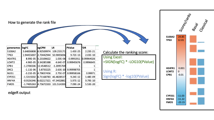
Generation of the rank file
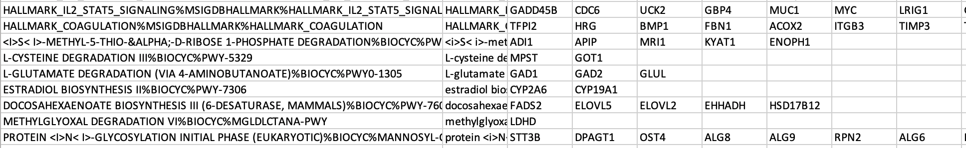
Select the gene names and score columns and save the file as tab delimited with the extension .rnk
![]()
Pathway defintion file
The second file that is needed for GSEA is the pathway database, a file with the .gmt extension. The pathway database (.gmt) used for the GSEA analysis was downloaded from http://baderlab.org/GeneSets. This file contains gene-sets obtained from MsigDB-c2 and Hallmarks, NCI, Biocarta, IOB, Netpath, HumanCyc, Reactome, Panther, Pathbank, WikiPathways and the Gene Ontology (GO) databases.
You don’t need to perform this step for the exercise, the .gmt file
will be given to you.
Go to:
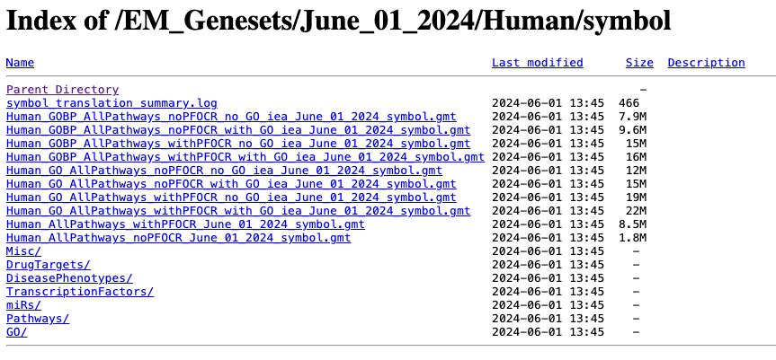
- http://download.baderlab.org/EM_Genesets/
- Click on June_01_2024/
- Click on Human/
- Click on symbol/
- Save the Human_GOBP_AllPathways_noPFOCR_no_GO_iea…gmt file on your computer
The .gmt is a tab delimited text file which contains one gene-set per row. For each gene-set (row), the first 2 columns contain the name and the description of the gene-set and the remaining columns contain the list of genes included in the gene-set. It is possible to create a custom gene-set using Excel or R.
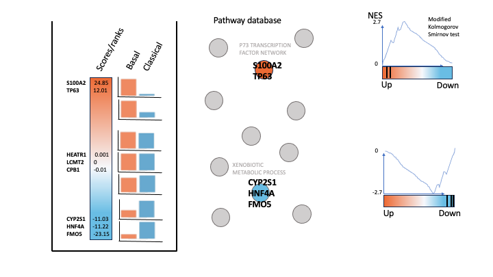
GSEA performs a gene-set enrichment analysis using a modified Kolmogorov-Smirnov statistic. The output result consists of summary tables displaying enrichment statistics for each gene-set (pathway) that has been tested.
Start the exercise
Before starting this exercise, download the 2 required files:
Right click on link below and select “Save Link As…”.
Place it in the corresponding module directory of your CBW work directory.
Step1.
Launch GSEA by double clicking on the installed program icon.
If GSEA won’t launch on MacOS. (This is relevant for MacOS users on older operating systems. As I am not longer on this operating system I can’t regenerate these screenshots so they reflect an older version of GSEA but the steps are still relelvant if you are working on Catalina with the latest version of GSEA)
Follow instructions specified on download page: * 
-
If you see this error message:
-
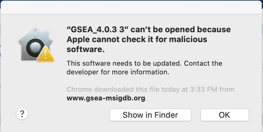
-
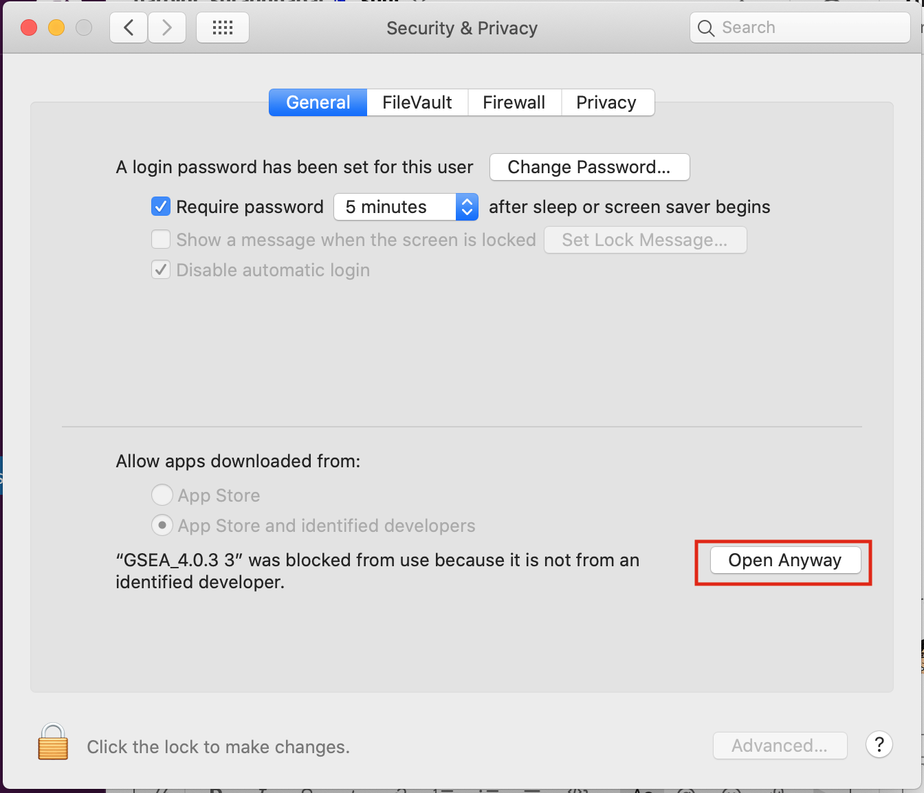
Open Settings -> Security & Privacy
-
Click on “Open Anyways”
-
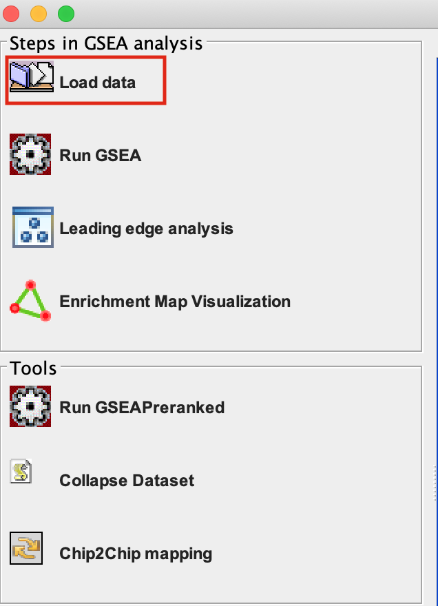
Step 2.
Load Data
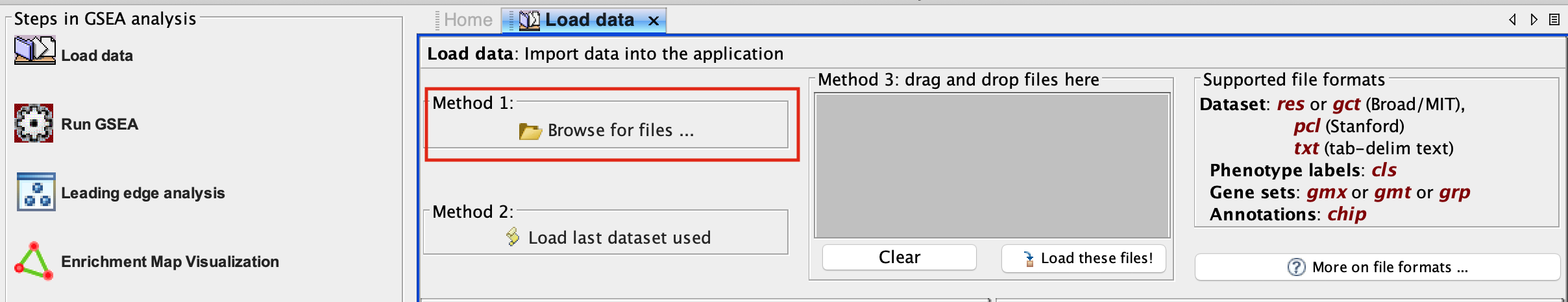
2a. Locate the ‘Load data’ icon at the upper left corner of the window and click on it.
2b. In the central panel, select ‘Method 1’ and ‘Browse for files’. A new window pops up.
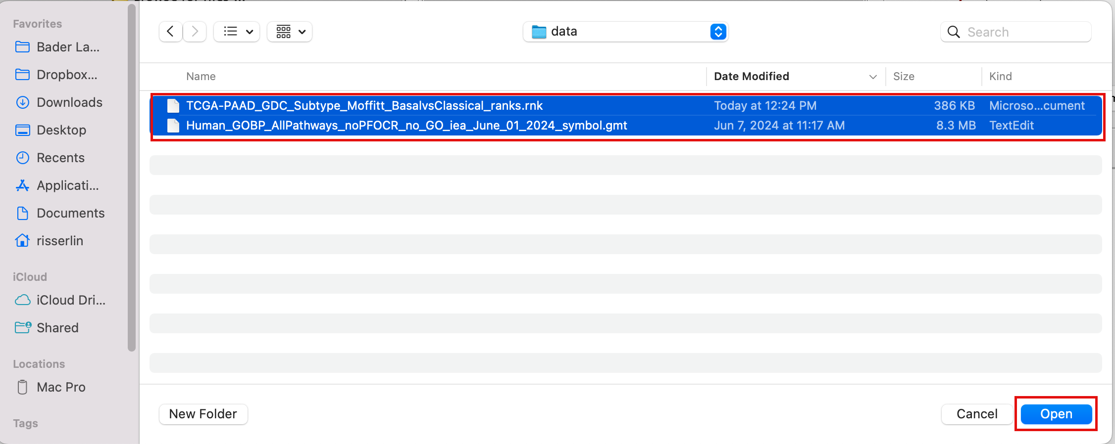
2c. Browse your computer to locate and select the 2 files : Human_GOBP_AllPathways_noPFOCR_no_GO_iea_June_01_2024_symbol.gmt and TCGA-PAAD_GDC_Subtype_Moffitt_BasalvsClassical_ranks.rnkk.
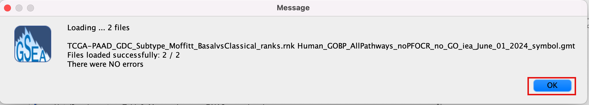
2d. Click on Open. A message pops us when the files are loaded successfully.
2e. Click on OK.
Alternatively, you can choose Method 3 to drag and drop files here. You need to click on the Load these files! button in this case.
Step3.
Adjust parameters
3a. Under the Tools menu select GseaPreRanked.
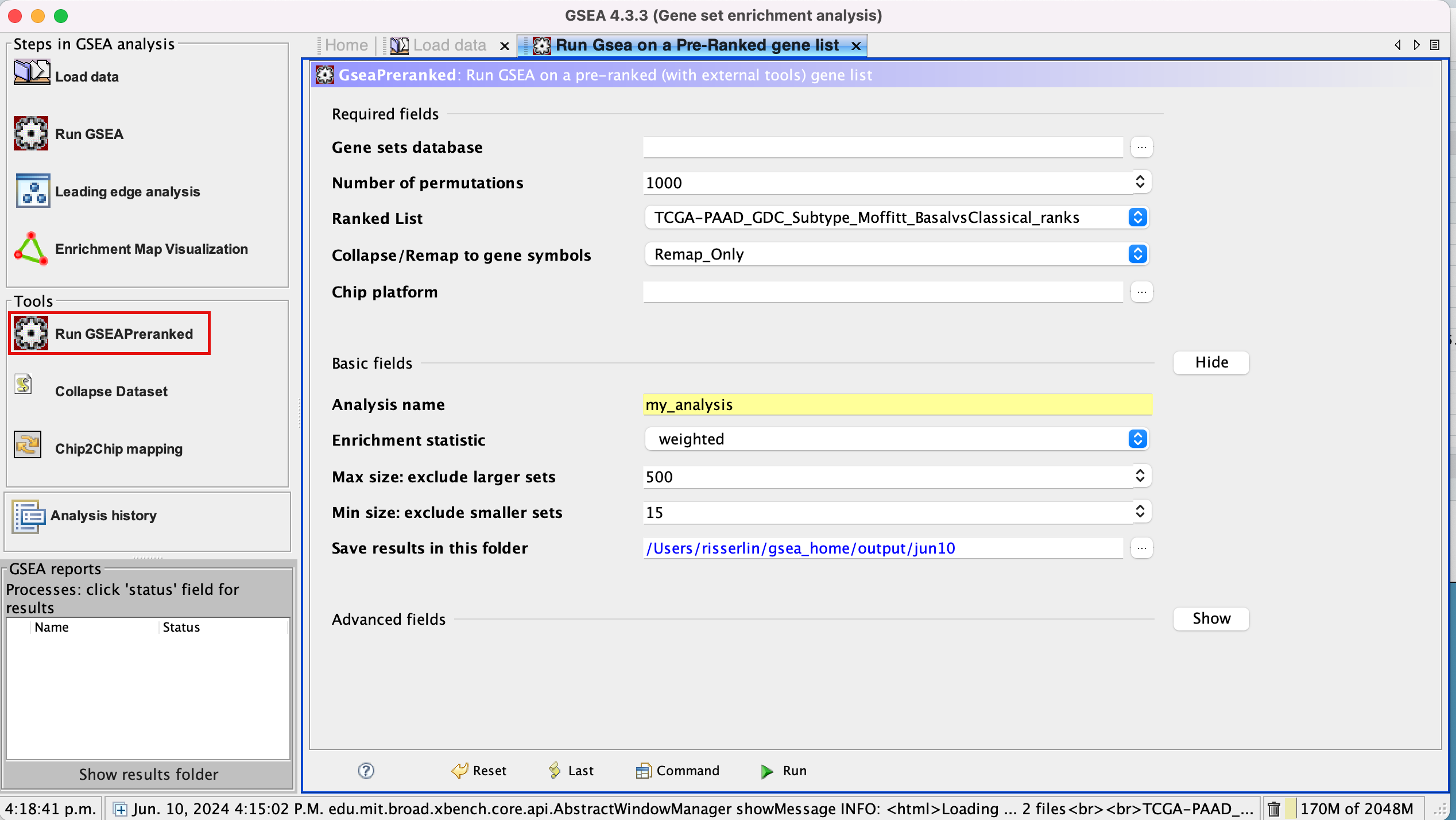
3b. Run GSEA on a Pre-Ranked gene list tab will appear.
Specify the following parameters:
3c. Gene sets database -
- Click on the radio button (…) located at the right of the blank field.
- Wait 5-10 sec for the gene-set selection window to appear.
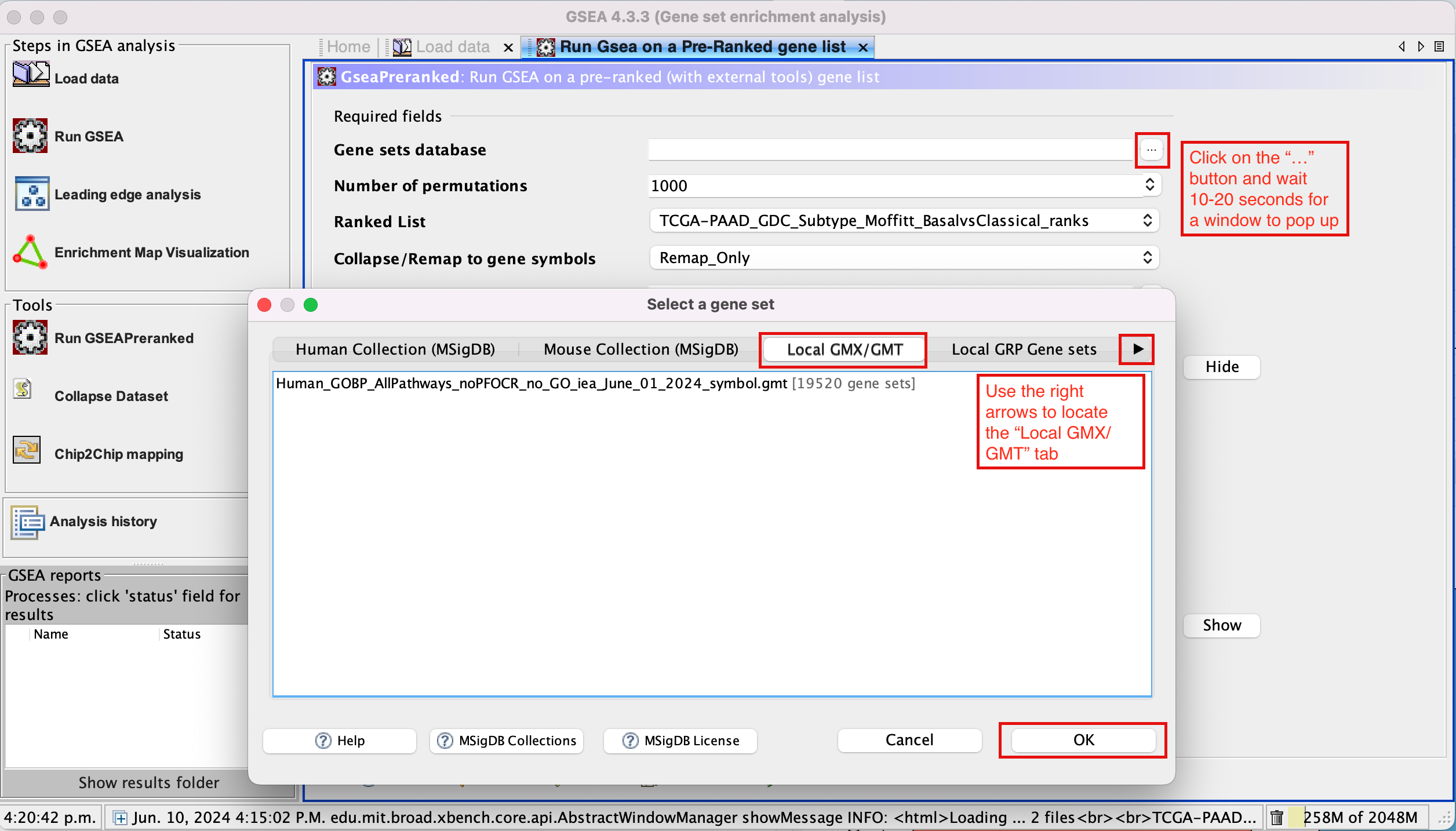
- Use the right arrow in the top field to see the Gene matrix (Local gmx/gmt) tab.
- Click to highlight Human_GOBP_AllPathways_noPFOCR_no_GO_iea_June_01_2024_symbol.gmt.
- Click on OK at the bottom of the window.
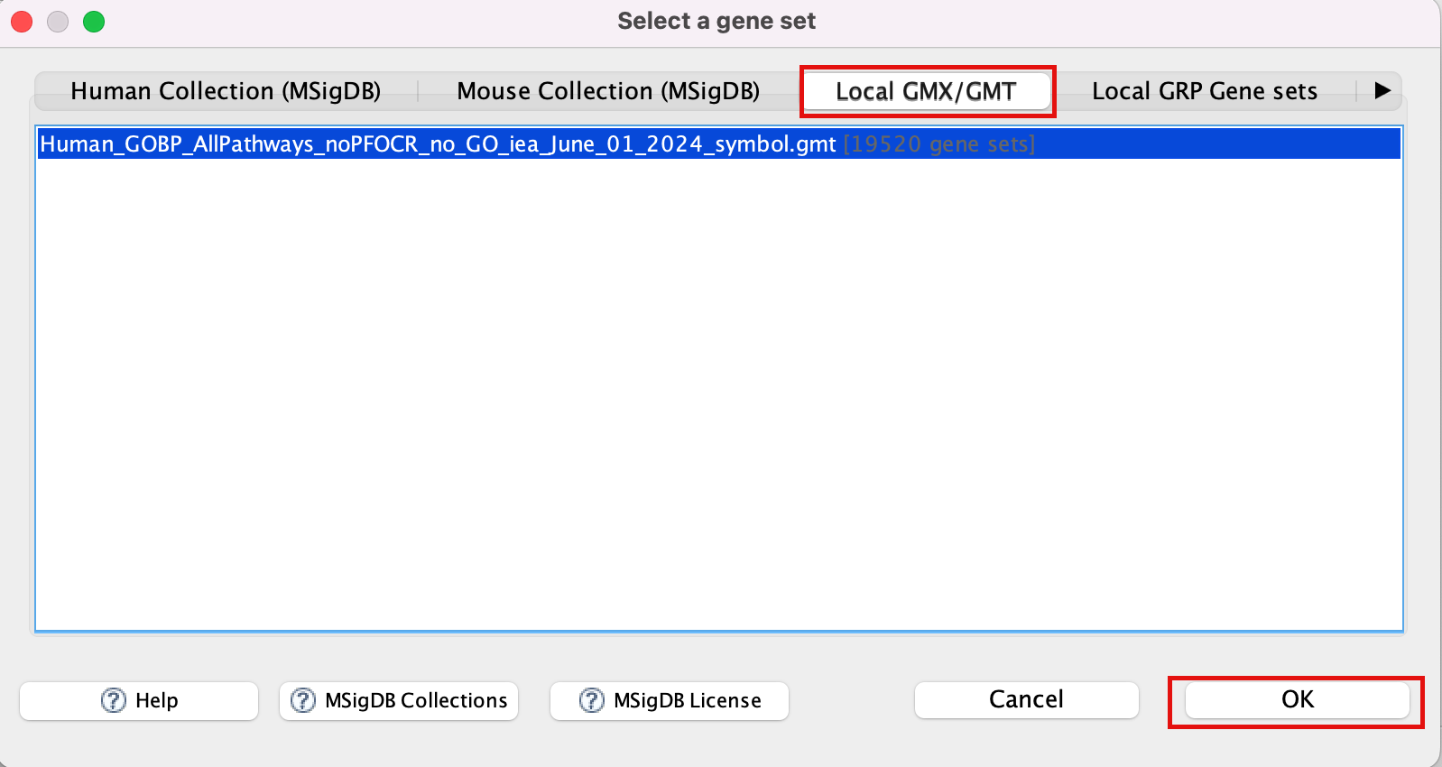
- Human_GOBP_AllPathways_noPFOCR_no_GO_iea_June_01_2024_symbol.gmt is now visible in the field corresponding to Gene sets database.
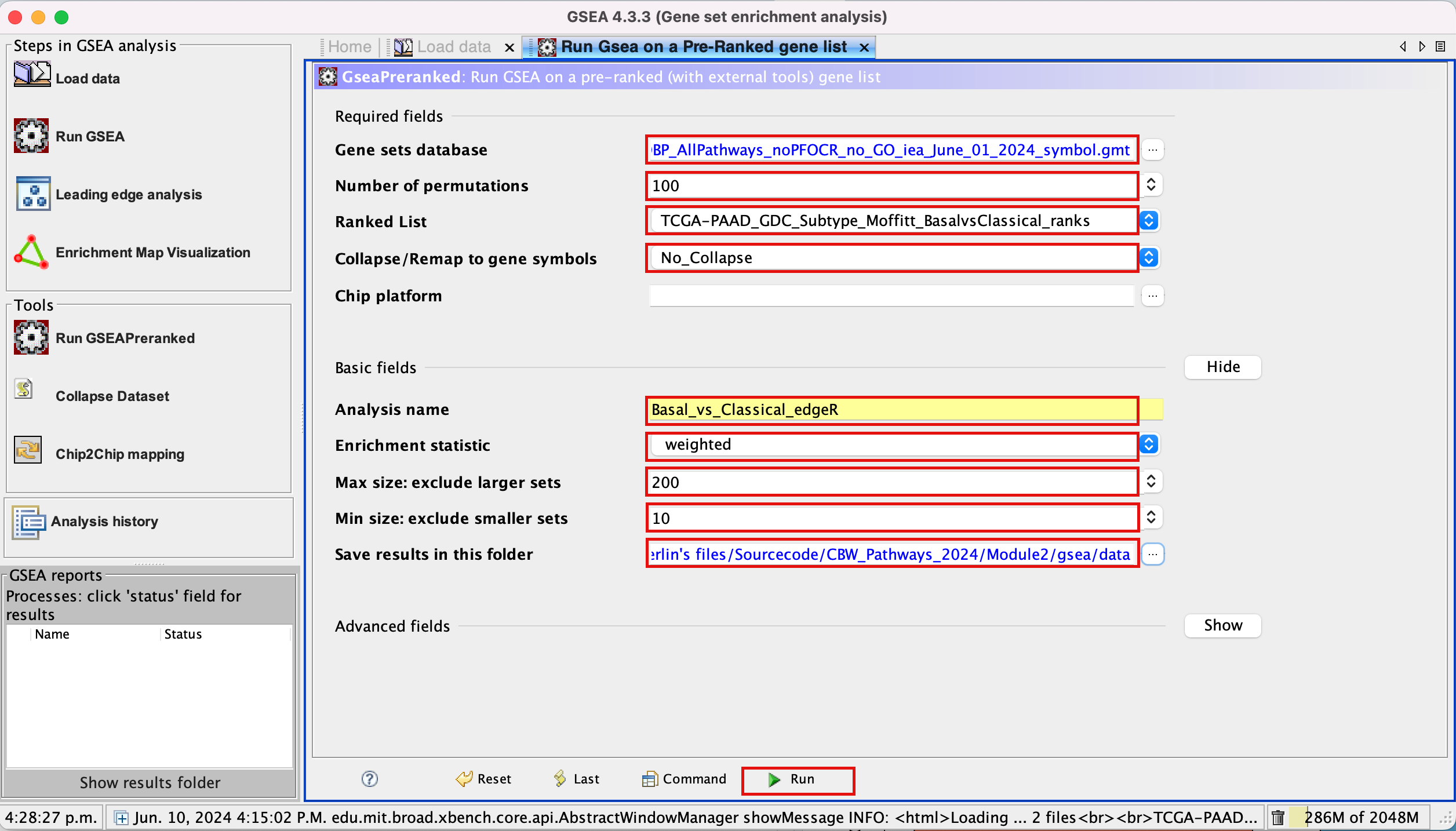
3d. Set Number of permutations to 100. The number of permutations is the number of times that the gene-sets will be randomized in order to create a null distribution to calculate the FDR.
Use 2000 when you do it for your own data outside the workshop.
3e. Ranked list - select by clicking on the arrow and highlighting rank file.
3f. Collapse/Remap to gene symbols - Change to No_collapse. (Our rank file already contains the gene symbols so we don’t need GSEA to try and convert probe names to gene symbols)
3g. Click on Show button next to Basic Fields to display extra options.
3h. Analysis name – change the default name my_analysis to a name that is specific to analysis. For example Basal_vs_Classical_edgeR. GSEA will use your specified name as part of the directory of results that it creates.
3i. Max size: exclude larger sets – By default GSEA sets the upper limit to 500. In this protocol, the maximum is set to 200 to decrease some of the larger sets in the results.
3j. Min size: exclude smaller sets – By default GSEA sets the lower limit to 15. In this protocol, the minimum is set to 10 to increase some of the smaller sets in the results.
3k. Save results in this folder – navigate to where you want GSEA to put the results folder. By default GSEA will put the results into the directory gsea_home/output/[date] in your home directory.
Set Enrichment Statistics to p2 if you want to add
more weight on the most top up-regulated and top down-regulated.
P2 is a more stringent parameter and it will result in
less gene-sets significant under FDR <0.05.
Step 4.
Run GSEA
4a. Click on Run button located at the bottom right corner of the window.
Expand the window size if the run button is not visible
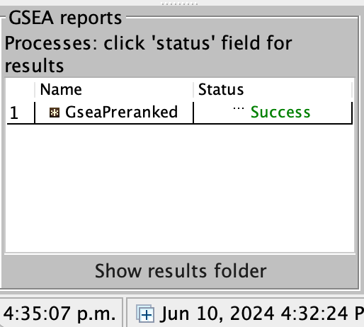
4b. On the panel located on the left side of the GSEA window, the bottom panel called GSEA report will show that a process was created, with a message that it is Running.
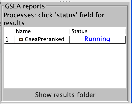
On completion the status message will be updated to Success….
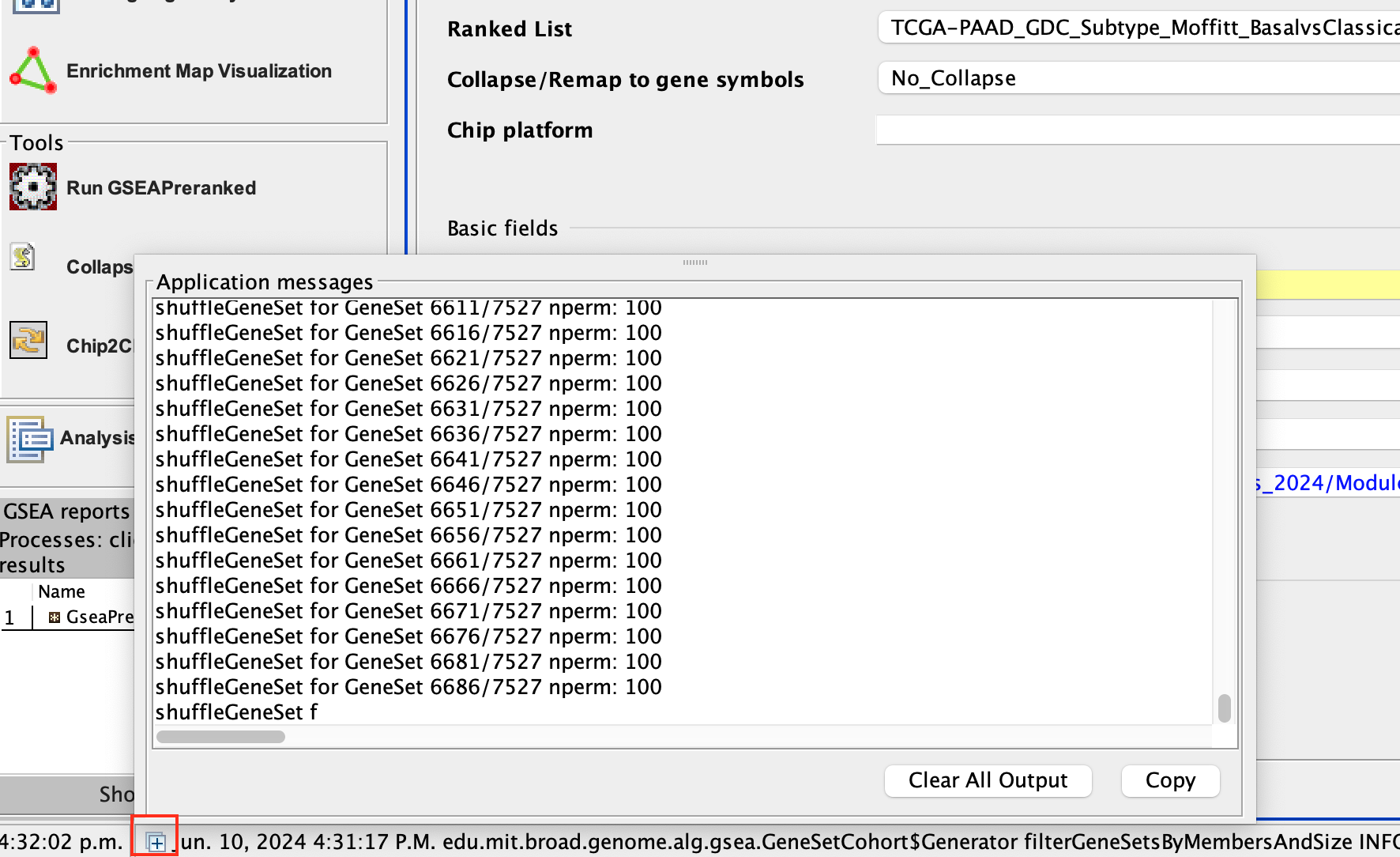
There is no progress bar to indicate to the user how much time is left to complete the process. Depending on the size of your dataset and compute power of your machine, a GSEA run can take from a few minutes to a few hours. To check on the status of the GSEA run in the bottom left hand corner you can click on the + (red circle in above Figure) to see the updating status. Printouts in the format shuffleGeneSet for GeneSet 5816/6878 nperm: 100 indicate how many permutations have been done (5816) out of the total that need to be performed (6878).
If the permutations have been completed but the status is still running, it means that GSEA is creating the report
Java Heap Space error. If GSEA returns an error Java Heap space it means that GSEA has run out of memory. If you are running GSEA from the webstart other than the 4GB option, then you will need to download a new version that allows for more memory allocation. The current maximum memory allocation that the GSEA webstart allows for is 4GB. If you are using this version and still receive the java heap error, you will need to download the GSEA java jar file and launch it from the command line as described in step 1.
Step 5.
Examining the results
5a. Click on Success to launch the results in html format in your default web browser.
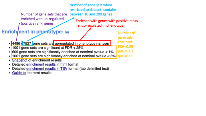
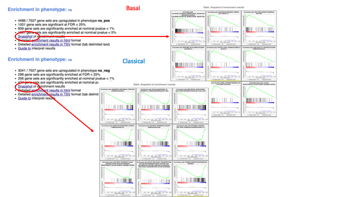
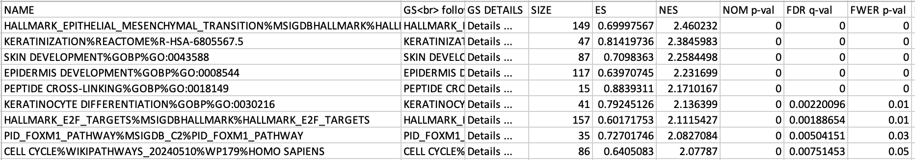
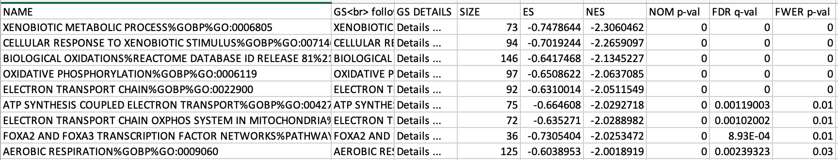
If the GSEA application has been closed, you can still see the results by opening the result folder and clicking on the index file – index.html. (see screenshot below). The first phenotype corresponds to gene-sets enriched in genes up-regulated in the Basal subtype. The second phenotype corresponds to gene-sets enriched in genes up-regulated in the Classical phenotype.
When examining the results there are a few things to look for:
5b. Check the number of gene-sets that have been used for the analysis.
A small number (a few hundred genesets if using baderlab genesets) could indicate an issue with identifier mapping.
5c. Check the number of sets that have FDR less than 0.25 – in order to determine what thresholds to start with when creating the enrichment map. It is not uncommon to see a thousand gene sets pass the threshold of FDR less than 0.25. FDR less than 0.25 is a very lax threshold and for robust data we can set thresholds of FDR less than 0.05 or lower.
5d. Click on Snapshots to see the trend for the top 20 genesets. For the positive phenotype the top genesets should show a distribution skewed to the left (positive) i.e. genesets have predominance of up-regulated genes. For the negative phenotype the top geneset should be inverted and skewed to the right (negative) i.e. geneset have predominance of down-regulated genes.
5e. Explore the tabular format of the results.
Additional information
More on processing the RNAseq using EdgeR and generate the .rank file
More on which .gmt file to download from the Baderlab gene-set file, select current release, Human, symbol, Human_GOBP_AllPathways_no_GO_iea_….gmt
Bonus - Automation.
Run analysis directly from R for easy integration into existing pipelines.
Instead of using the GSEA application you can run it directly from R using the GSEA java jar that can be easily used within the workshop docker image (workshop_base_image) that you setup duing your prework.
Follow the step by step instructions on how to run from R here - https://risserlin.github.io/CBW_pathways_workshop_R_notebooks/run-gsea-from-within-r.html
First, make sure your environment is set up correctly by following there instructions - https://risserlin.github.io/CBW_pathways_workshop_R_notebooks/setup.html