Module 8.4 Lab: BYOD - Differential Expression (Palbo-resistant vs Abema-resistant)

This work is licensed under a Creative Commons Attribution-ShareAlike 4.0 Unported License. This means that you are able to copy, share and modify the work, as long as the result is distributed under the same license.

We perform differential expression analysis comparing the Palbo-resistant and the Abema-resistant MCF7 cell lines using a negative binomial generalized linear model using the edgeR package.

Install and load libraries

## CRAN and Bioconductor setup
if (!requireNamespace("BiocManager", quietly = TRUE))
  install.packages("BiocManager")

## List of CRAN packages
cran_packages <- c(
  "tidyverse",
  "ggrepel"
)

# List of Bioconductor packages
bioc_packages <- c(
  "edgeR"
)

# Install CRAN packages if not already installed
for (pkg in cran_packages) {
  if (!requireNamespace(pkg, quietly = TRUE)) {
    install.packages(pkg)
  }
}

# Install Bioconductor packages if not already installed
for (pkg in bioc_packages) {
  if (!requireNamespace(pkg, quietly = TRUE)) {
    BiocManager::install(pkg)
  }
}

# Load the libraries

# CRAN packages
library(tidyverse)
library(ggrepel)
# Bioconductor packages
library(edgeR)

# create the results folder (if it does not exist yet) to save the outputs
# dir.create("results", showWarnings = FALSE)

# Location of the Module 8 files (data/, BYODdata/, image/):
# - on the course server: ~/CourseData/Module8
# - when the book is built from the repository: Module8
data_dir <- if (dir.exists("~/CourseData/Module8")) "~/CourseData/Module8" else "Module8"

Data used for this comparison

For this analysis, we are going to compare the Palbo-resistant cell lines (MCF7 1.2 Palbo-resistant, 3 biological replicates) versus the Abema-resistant cell lines (MCF7 0.5 Abema-resistant, 3 biological replicates). The count files are in the BYODdata folder.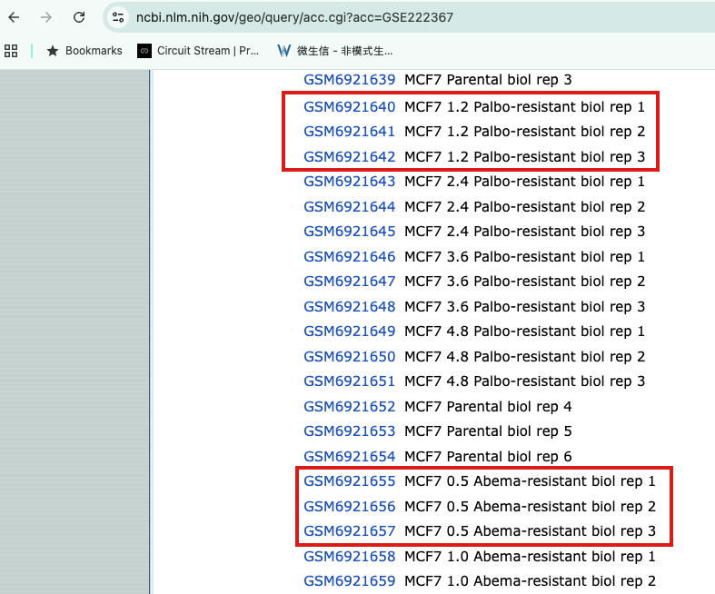

Figure 4: GEO dataset (GSE222367): samples used for the Palbo-resistant vs Abema-resistant comparison

generate a DGE object

# 1. Find the count files
files <- list.files(path = file.path(data_dir, "BYODdata"), pattern = "\\.txt\\.gz$", full.names = TRUE)

# 2. Sample names from the file names (strip the extension)
samples <- sub("_S.*", "", basename(files))

# 3. Read the files into a DGEList
#    HTSeq output has no header: column 1 = gene ID, column 2 = count.
#    R reads gzipped files directly, so no need to decompress.
dge <- readDGE(files, columns = c(1, 2), header = FALSE, labels = samples)

## Meta tags detected: __no_feature, __ambiguous, __too_low_aQual, __not_aligned, __alignment_not_unique

# 4. Remove HTSeq summary rows (__no_feature, __ambiguous, etc.)
dge <- dge[!grepl("^__", rownames(dge)), , keep.lib.sizes = FALSE]

# 5. (Optional) add group information
#    files are listed in this order: GSM6921640-42 (Palbo-resistant),
#    then GSM6921655-57 (Abema-resistant)
dge$samples$group <- factor(
  c("palbo_resistant", "palbo_resistant", "palbo_resistant",
    "abema_resistant", "abema_resistant", "abema_resistant"),
  levels = c("abema_resistant", "palbo_resistant")   # abema_resistant = reference
)

# check that each sample has the right group
dge$samples[, c("files", "group")]

##                                                             files
## GSM6921640 Module8/BYODdata/GSM6921640_S1M712_P.htseqcount.txt.gz
## GSM6921641 Module8/BYODdata/GSM6921641_S5M712_P.htseqcount.txt.gz
## GSM6921642 Module8/BYODdata/GSM6921642_S6M712_P.htseqcount.txt.gz
## GSM6921655 Module8/BYODdata/GSM6921655_S2M705_A.htseqcount.txt.gz
## GSM6921656 Module8/BYODdata/GSM6921656_S3M705_A.htseqcount.txt.gz
## GSM6921657 Module8/BYODdata/GSM6921657_S4M705_A.htseqcount.txt.gz
##                      group
## GSM6921640 palbo_resistant
## GSM6921641 palbo_resistant
## GSM6921642 palbo_resistant
## GSM6921655 abema_resistant
## GSM6921656 abema_resistant
## GSM6921657 abema_resistant

Filter low-count genes and TMM-normalize

keep <- filterByExpr(dge, group = dge$samples$group)
dge  <- dge[keep, , keep.lib.sizes = FALSE]
dge  <- calcNormFactors(dge, method = "TMM")

## calcNormFactors has been renamed to normLibSizes

cat("Genes retained after filtering:", nrow(dge), "\n")

## Genes retained after filtering: 13488

mds <- plotMDS(dge, col = as.numeric(dge$samples$group), main = "MDS (logCPM)")

group = dge$samples$group
var_pct <- round(100 * mds$var.explained[mds$dim.plot])
mds_df <- data.frame(dim1 = mds$x, dim2 = mds$y,
                      sample = colnames(dge), group = group)

ggplot(mds_df, aes(x = dim1, y = dim2, color = group)) +
  geom_point(size = 3) +
  ggrepel::geom_text_repel(aes(label = sample), size = 3, color = "grey30",
                            show.legend = FALSE, max.overlaps = Inf,
                            box.padding = 0.4, segment.color = "grey60") +
  labs(title = "MDS plot (all samples)",
       x = sprintf("Leading logFC dim %d (%d%%)", mds$dim.plot[1], var_pct[1]),
       y = sprintf("Leading logFC dim %d (%d%%)", mds$dim.plot[2], var_pct[2]),
       color = "Group") +
  theme_minimal(base_size = 12) +
  theme(legend.position = "right")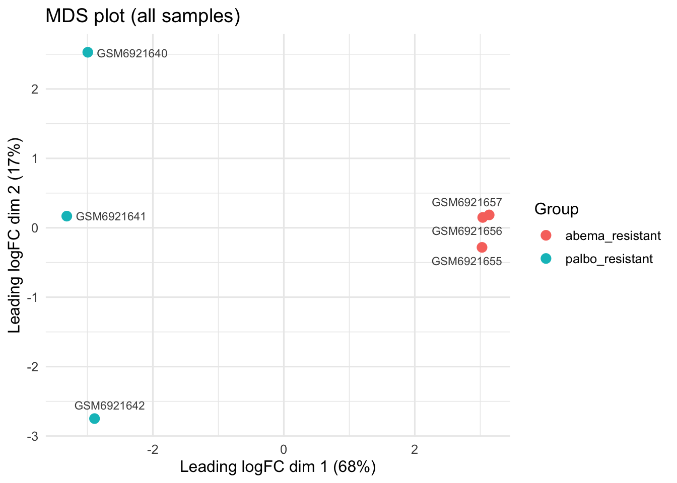

Design (~0 + group) and named contrast

design <- model.matrix(~ 0 + group, data = dge$samples)
colnames(design) <- levels(dge$samples$group)   # "abema_resistant", "palbo_resistant"

contr <- makeContrasts(
  palbo_resistant_vs_abema_resistant = palbo_resistant - abema_resistant,   # + logFC = up in Palbo-resistant
  levels = design
)

head(design)

##            abema_resistant palbo_resistant
## GSM6921640               0               1
## GSM6921641               0               1
## GSM6921642               0               1
## GSM6921655               1               0
## GSM6921656               1               0
## GSM6921657               1               0

Dispersion estimation and quasi-likelihood GLM

dge <- estimateDisp(dge, design, robust = TRUE)
fit <- glmQLFit(dge, design, robust = TRUE)
 
par(mfrow = c(1, 2)); plotBCV(dge); plotQLDisp(fit)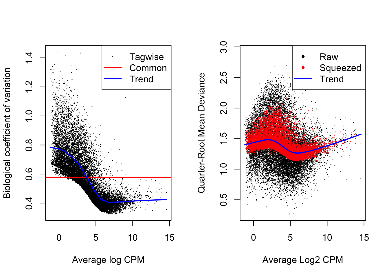

qlf <- glmQLFTest(fit, contrast = contr[, "palbo_resistant_vs_abema_resistant"])
 
res <- topTags(qlf, n = Inf, sort.by = "PValue")$table
res$gene <- rownames(res)

Calculating ranking score and export full results

res$score = sign(res$logFC) * -log10(res$PValue)
head(res)

##            logFC   logCPM        F       PValue          FDR  gene      score
## AZGP1 -12.702093 8.537657 393.9245 4.359694e-12 5.880356e-08 AZGP1 -11.360544
## EPN3  -12.159764 7.082619 276.4453 2.148481e-10 1.448936e-06  EPN3  -9.667868
## CLDN7 -10.436250 5.736231 211.5922 4.527979e-10 2.035780e-06 CLDN7  -9.344096
## CSTA   -9.803252 5.643118 185.4895 8.772884e-10 2.744236e-06  CSTA  -9.056858
## BST2   -9.397769 6.194576 236.5503 1.017288e-09 2.744236e-06  BST2  -8.992556
## PKP1  -10.368285 6.594349 187.1473 1.442829e-09 3.243480e-06  PKP1  -8.840785

##visualization

### histogram of the ranking score
hist(res$score, breaks=100, col="orchid", xlab = "score", main = "Histogram of score")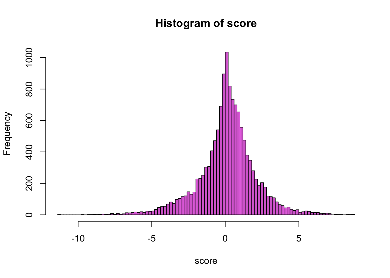

### volcano plot

# Step 1: add -log10(FDR), and label each gene Up / Down / Not sig
res <- res %>%
  mutate(
    negLogFDR = -log10(FDR),
    status = case_when(
      FDR < 0.05 & logFC > 0 ~ "Up",
      FDR < 0.05 & logFC < 0 ~ "Down",
      TRUE ~ "Not sig"
    )
  )

# Step 2: pick the top 15 most significant genes on each side, to label
top_up   <- res %>% filter(status == "Up")   %>% arrange(FDR) %>% slice_head(n = 15)
top_down <- res %>% filter(status == "Down") %>% arrange(FDR) %>% slice_head(n = 15)
top_genes <- bind_rows(top_up, top_down)

# Step 3: plot
ggplot(res, aes(x = logFC, y = negLogFDR, color = status)) +
  geom_point() +
  scale_color_manual(values = c("Up" = "#D55E00", "Down" = "#0072B2", "Not sig" = "grey")) +
 ggrepel::geom_text_repel(data = top_genes, aes(label = gene), max.overlaps = Inf) +
  labs(title = "Palbo-resistant vs Abema-resistant",
       subtitle = "Up = higher in Palbo-resistant, Down = higher in Abema-resistant",
       x = "log2 Fold Change", y = "-log10(FDR)", color = "Status")+
  coord_cartesian(ylim = c(0, 4.5)) +
  theme_classic()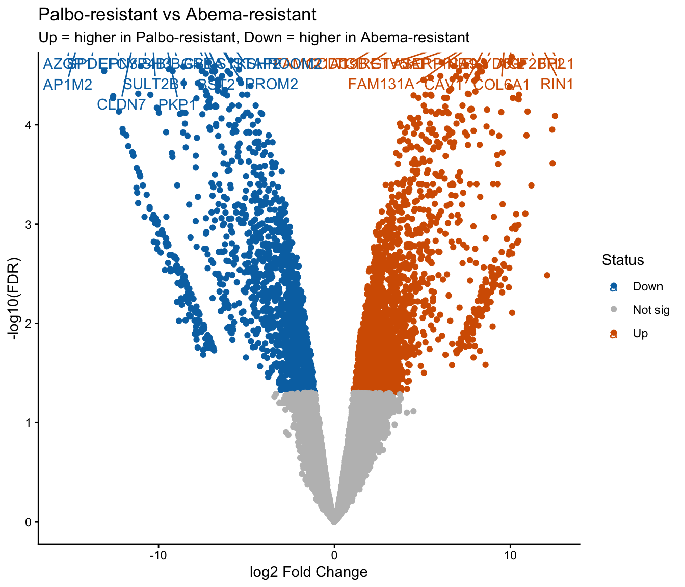

Result output

print(summary(decideTests(qlf, adjust.method = "BH", p.value = 0.05)))

##        -1*abema_resistant 1*palbo_resistant
## Down                                   1608
## NotSig                                10036
## Up                                     1844

# write.csv(res, "results/edgeR_palbo_resistant_vs_abema_resistant_all_genes.csv", row.names = FALSE)

YOUR TURN

Now use the differential expressed genes and perform pathway enrichment analysis using g:Profiler or fgsea as described in Module 8

Additional exercise

Use the genes from Module 5 (BRCA1, BRCA2 and TP53) and build a protein protein interaction network with the String All in Cytoscape and discover their shared interactors. Perform pathway enrichment analysis on the created network.

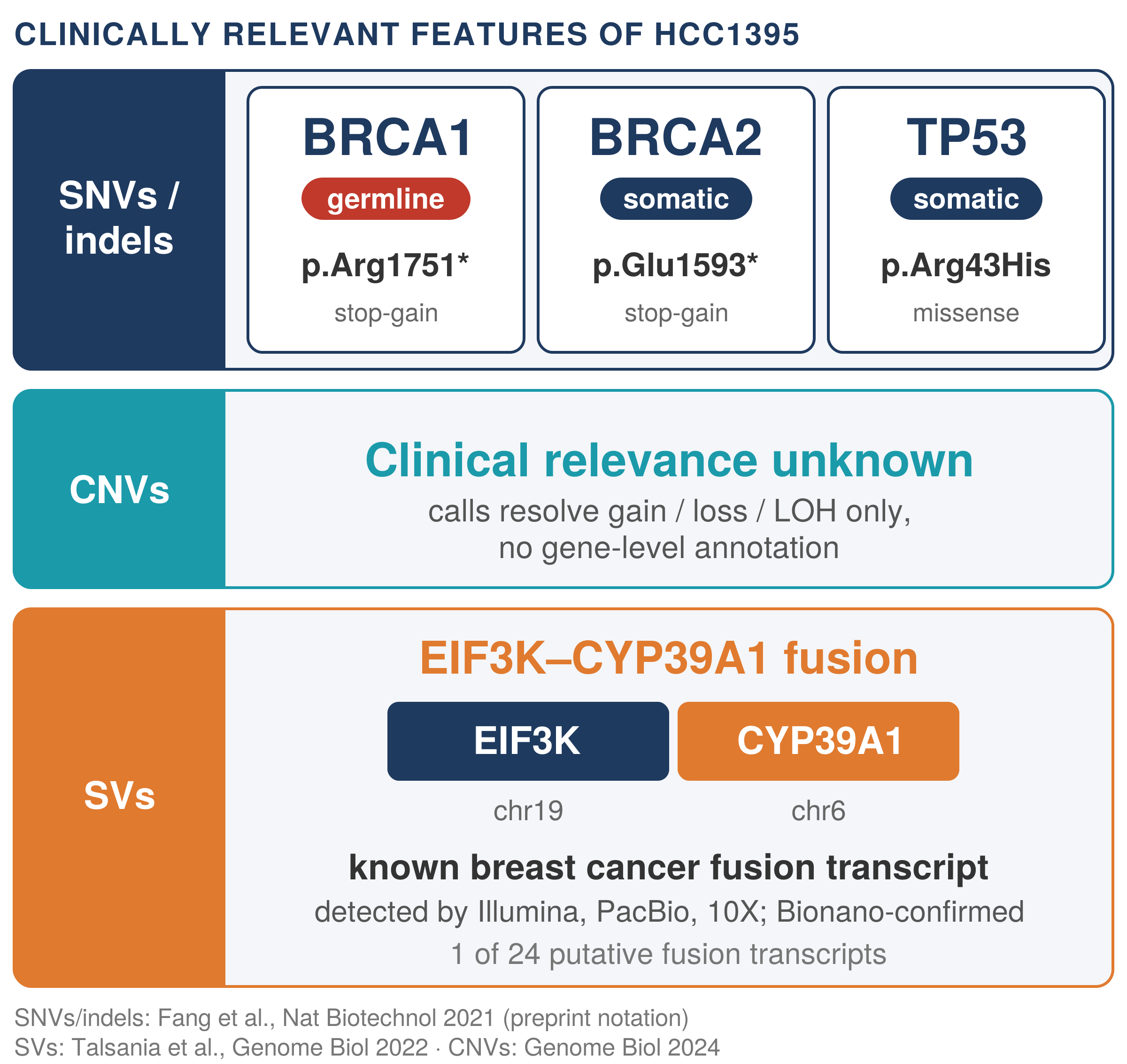
Clinically relevant features of HCC1395 (Module 5): BRCA1 germline stop-gain, BRCA2 somatic stop-gain and TP53 somatic missense mutations, and the EIF3K-CYP39A1 fusion transcript.

Figure 5: Clinically relevant features of HCC1395 (Module 5): BRCA1 germline stop-gain, BRCA2 somatic stop-gain and TP53 somatic missense mutations, and the EIF3K-CYP39A1 fusion transcript.

Query the 3 genes with the STRING protein query in Cytoscape (species Homo sapiens, full STRING network, confidence score cutoff 0.40, maximum 30 additional interactors).

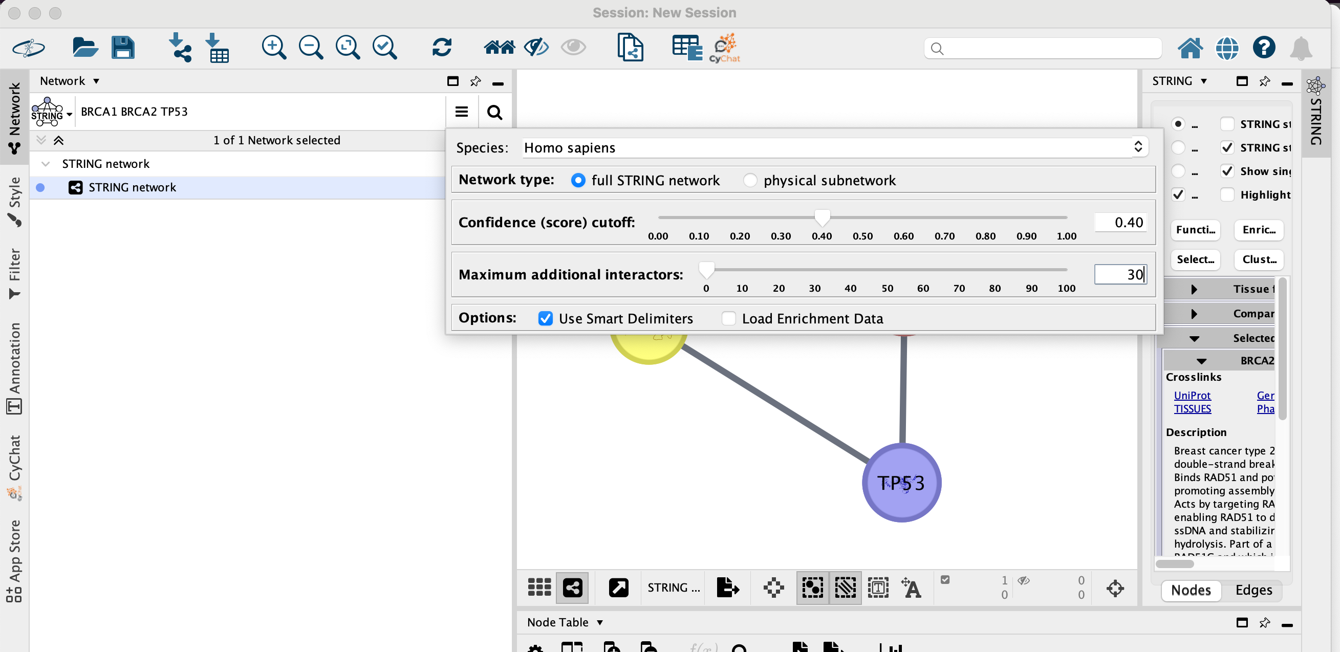
Figure 6: STRING protein query in Cytoscape with BRCA1, BRCA2 and TP53.

The resulting network contains the 3 genes and their shared interactors. Run the STRING functional enrichment to see which pathways are enriched in the network.

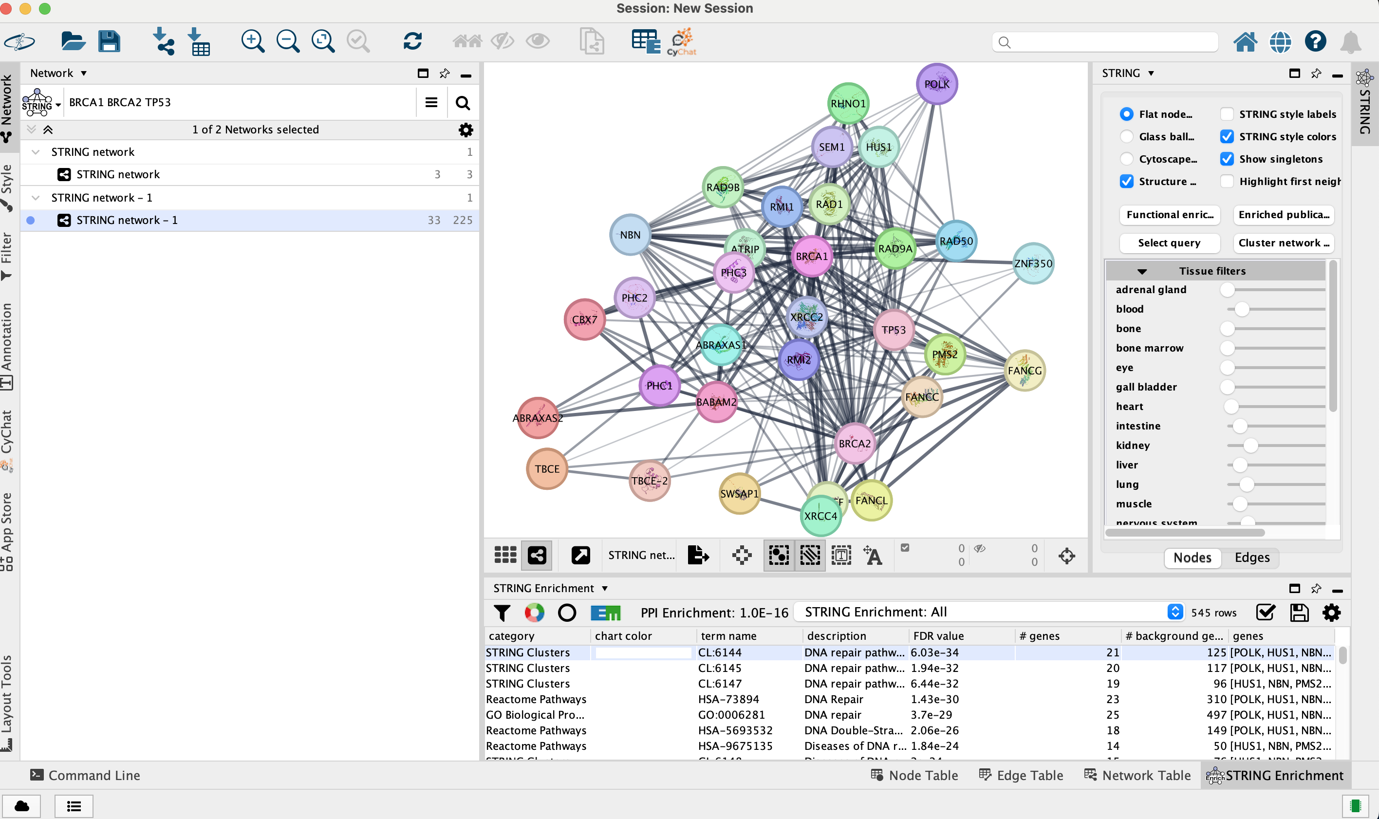
STRING network of BRCA1, BRCA2, TP53 and their interactors (33 nodes, 225 edges), with the STRING enrichment table: DNA repair pathways are the most enriched.

Figure 7: STRING network of BRCA1, BRCA2, TP53 and their interactors (33 nodes, 225 edges), with the STRING enrichment table: DNA repair pathways are the most enriched.