Module 8.1 Lab: Differential Expression

This work is licensed under a Creative Commons Attribution-ShareAlike 4.0 Unported License. This means that you are able to copy, share and modify the work, as long as the result is distributed under the same license.

We perform differential expression analysis using a negative binomial generalized linear model using the edgeR package.

Install and load libraries

## CRAN and Bioconductor setup
if (!requireNamespace("BiocManager", quietly = TRUE))
  install.packages("BiocManager")

## List of CRAN packages
cran_packages <- c(
  "tidyverse",
  "ggrepel"
)

# List of Bioconductor packages
bioc_packages <- c(
  "edgeR"
)

# Install CRAN packages if not already installed
for (pkg in cran_packages) {
  if (!requireNamespace(pkg, quietly = TRUE)) {
    install.packages(pkg)
  }
}

# Install Bioconductor packages if not already installed
for (pkg in bioc_packages) {
  if (!requireNamespace(pkg, quietly = TRUE)) {
    BiocManager::install(pkg)
  }
}

# Load the libraries

# CRAN packages
library(tidyverse)

## ── Attaching core tidyverse packages ────────────────────
## ✔ dplyr     1.2.1     ✔ purrr     1.2.2
## ✔ forcats   1.0.1     ✔ stringr   1.6.0
## ✔ ggplot2   4.0.3     ✔ tibble    3.3.1
## ✔ lubridate 1.9.5     ✔ tidyr     1.3.2
## ── Conflicts ─────────────────── tidyverse_conflicts() ──
## ✖ dplyr::filter()  masks stats::filter()
## ✖ purrr::flatten() masks jsonlite::flatten()
## ✖ dplyr::lag()     masks stats::lag()
## ℹ Use the conflicted package (<http://conflicted.r-lib.org/>) to force all conflicts to become errors

library(ggrepel)
# Bioconductor packages
library(edgeR)

## Loading required package: limma

# create the results folder (if it does not exist yet) to save the outputs
# dir.create("results", showWarnings = FALSE)

# Location of the Module 8 files (data/, BYODdata/, image/):
# - on the course server: ~/CourseData/Module8
# - when the book is built from the repository: Module8
data_dir <- if (dir.exists("~/CourseData/Module8")) "~/CourseData/Module8" else "Module8"

Data used for this comparison

For this analysis, we are going to compare the Palbo-resistant cell lines (3 biological replicates) versus the parental cell lines (3 biological replicates)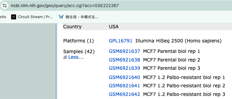

Figure 2: GEO dataset

generate a DGE object

# 1. Find the count files
files <- list.files(path = file.path(data_dir, "data"), pattern = "\\.txt\\.gz$", full.names = TRUE)

# 2. Sample names from the file names (strip the extension)
samples <- sub("_S.*", "", basename(files))

# 3. Read the files into a DGEList
#    HTSeq output has no header: column 1 = gene ID, column 2 = count.
#    R reads gzipped files directly, so no need to decompress.
dge <- readDGE(files, columns = c(1, 2), header = FALSE, labels = samples)

## Meta tags detected: __no_feature, __ambiguous, __too_low_aQual, __not_aligned, __alignment_not_unique

# 4. Remove HTSeq summary rows (__no_feature, __ambiguous, etc.)
dge <- dge[!grepl("^__", rownames(dge)), , keep.lib.sizes = FALSE]

# 5. (Optional) add group information
dge$samples$group <- factor(
  c("parental", "parental", "parental",
    "palbo_resistant", "palbo_resistant", "palbo_resistant"),
  levels = c("parental", "palbo_resistant")   # parental = reference
)

Filter low-count genes and TMM-normalize

keep <- filterByExpr(dge, group = dge$samples$group)
dge  <- dge[keep, , keep.lib.sizes = FALSE]
dge  <- calcNormFactors(dge, method = "TMM")

## calcNormFactors has been renamed to normLibSizes

cat("Genes retained after filtering:", nrow(dge), "\n")

## Genes retained after filtering: 15246

mds <- plotMDS(dge, col = as.numeric(dge$samples$group), main = "MDS (logCPM)")

group = dge$samples$group
var_pct <- round(100 * mds$var.explained[mds$dim.plot])
mds_df <- data.frame(dim1 = mds$x, dim2 = mds$y,
                      sample = colnames(dge), group = group)

ggplot(mds_df, aes(x = dim1, y = dim2, color = group)) +
  geom_point(size = 3) +
  ggrepel::geom_text_repel(aes(label = sample), size = 3, color = "grey30",
                            show.legend = FALSE, max.overlaps = Inf,
                            box.padding = 0.4, segment.color = "grey60") +
  labs(title = "MDS plot (all samples)",
       x = sprintf("Leading logFC dim %d (%d%%)", mds$dim.plot[1], var_pct[1]),
       y = sprintf("Leading logFC dim %d (%d%%)", mds$dim.plot[2], var_pct[2]),
       color = "Group") +
  theme_minimal(base_size = 12) +
  theme(legend.position = "right")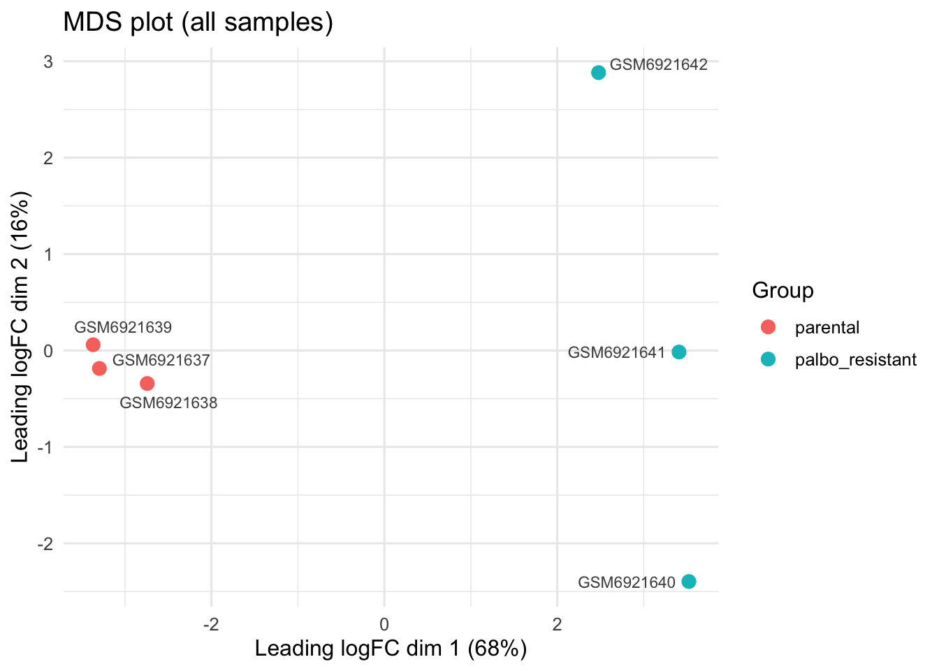

Design (~0 + group) and named contrast

design <- model.matrix(~ 0 + group, data = dge$samples)
colnames(design) <- levels(dge$samples$group)   # "parental", "palbo_resistant"
 
contr <- makeContrasts(
  resistant_vs_parental = palbo_resistant - parental,   # + logFC = up in resistant
  levels = design
)

head(design)

##            parental palbo_resistant
## GSM6921637        1               0
## GSM6921638        1               0
## GSM6921639        1               0
## GSM6921640        0               1
## GSM6921641        0               1
## GSM6921642        0               1

Dispersion estimation and quasi-likelihood GLM

dge <- estimateDisp(dge, design, robust = TRUE)
fit <- glmQLFit(dge, design, robust = TRUE)
 
par(mfrow = c(1, 2)); plotBCV(dge); plotQLDisp(fit)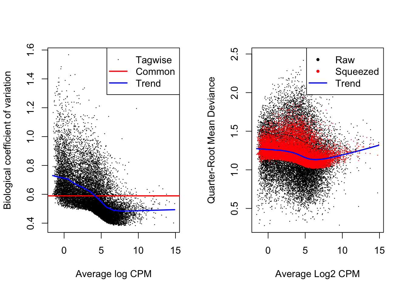

qlf <- glmQLFTest(fit, contrast = contr[, "resistant_vs_parental"])
 
res <- topTags(qlf, n = Inf, sort.by = "PValue")$table
res$gene <- rownames(res)

Calculating ranking score and export full results

res$score = sign(res$logFC) * -log10(res$PValue)
head(res)

##            logFC   logCPM        F       PValue          FDR  gene     score
## AZGP1 -11.100270 7.258554 210.7136 1.105697e-09 9.204042e-06 AZGP1 -8.956364
## EPN3  -11.063361 6.286707 178.1984 1.207404e-09 9.204042e-06  EPN3 -8.918147
## AP1M2 -12.060834 6.763487 162.9399 5.745195e-09 2.028808e-05 AP1M2 -8.240695
## SPDEF -12.276367 6.971532 157.8279 7.145788e-09 2.028808e-05 SPDEF -8.145950
## P3H2    9.908207 4.560450 136.4801 7.427137e-09 2.028808e-05  P3H2  8.129179
## SNTB1   8.362808 3.678316 140.8483 9.511283e-09 2.028808e-05 SNTB1  8.021761

##visualization

### histogram of the ranking score
hist(res$score, breaks=100, col="orchid", xlab = "score", main = "Histogram of score")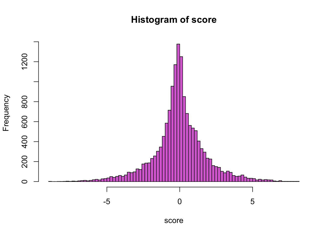

### volcano plot

# Step 1: add -log10(FDR), and label each gene Up / Down / Not sig
res <- res %>%
  mutate(
    negLogFDR = -log10(FDR),
    status = case_when(
      FDR < 0.05 & logFC > 0 ~ "Up",
      FDR < 0.05 & logFC < 0 ~ "Down",
      TRUE ~ "Not sig"
    )
  )

# Step 2: pick the top 15 most significant genes on each side, to label
top_up   <- res %>% filter(status == "Up")   %>% arrange(FDR) %>% slice_head(n = 15)
top_down <- res %>% filter(status == "Down") %>% arrange(FDR) %>% slice_head(n = 15)
top_genes <- bind_rows(top_up, top_down)

# Step 3: plot
ggplot(res, aes(x = logFC, y = negLogFDR, color = status)) +
  geom_point() +
  scale_color_manual(values = c("Up" = "#D55E00", "Down" = "#0072B2", "Not sig" = "grey")) +
 ggrepel::geom_text_repel(data = top_genes, aes(label = gene), max.overlaps = Inf) +
  labs(x = "log2 Fold Change", y = "-log10(FDR)", color = "Status")+
  coord_cartesian(ylim = c(0, 4.5)) +
  theme_classic()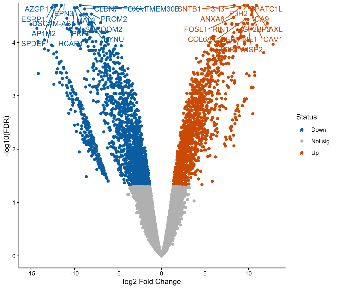

Result output

print(summary(decideTests(qlf, adjust.method = "BH", p.value = 0.05)))

##        -1*parental 1*palbo_resistant
## Down                            1652
## NotSig                         11986
## Up                              1608

# write.csv(res, "results/edgeR_resistant_vs_parental_all_genes.csv", row.names = FALSE)

Version of packages and R

sessionInfo()

## R version 4.6.1 (2026-06-24)
## Platform: aarch64-apple-darwin23
## Running under: macOS Tahoe 26.6
## 
## Matrix products: default
## BLAS:   /Library/Frameworks/R.framework/Versions/4.6/Resources/lib/libRblas.0.dylib 
## LAPACK: /Library/Frameworks/R.framework/Versions/4.6/Resources/lib/libRlapack.dylib;  LAPACK version 3.12.1
## 
## locale:
## [1] en_US.UTF-8/en_US.UTF-8/en_US.UTF-8/C/en_US.UTF-8/en_US.UTF-8
## 
## time zone: America/Toronto
## tzcode source: internal
## 
## attached base packages:
## [1] stats     graphics  grDevices utils     datasets  methods   base     
## 
## other attached packages:
##  [1] edgeR_4.10.7    limma_3.68.5    ggrepel_0.9.8   lubridate_1.9.5
##  [5] forcats_1.0.1   stringr_1.6.0   dplyr_1.2.1     purrr_1.2.2    
##  [9] tidyr_1.3.2     tibble_3.3.1    ggplot2_4.0.3   tidyverse_2.0.0
## [13] htmltools_0.5.9 jsonlite_2.0.0  readr_2.2.0    
## 
## loaded via a namespace (and not attached):
##  [1] sass_0.4.10         generics_0.1.4      stringi_1.8.9      
##  [4] lattice_0.23-1      hms_1.1.4           digest_0.6.39      
##  [7] magrittr_2.0.5      timechange_0.4.0    evaluate_1.0.5     
## [10] grid_4.6.1          RColorBrewer_1.1-3  bookdown_0.48      
## [13] fastmap_1.2.0       BiocManager_1.30.27 scales_1.4.0       
## [16] jquerylib_0.1.4     cli_3.6.6           rlang_1.3.0        
## [19] crayon_1.5.3        bit64_4.8.6         withr_3.0.3        
## [22] cachem_1.1.0        yaml_2.3.12         otel_0.2.0         
## [25] tools_4.6.1         parallel_4.6.1      tzdb_0.5.0         
## [28] locfit_1.5-9.12     vctrs_0.7.3         R6_2.6.1           
## [31] lifecycle_1.0.5     bit_4.6.0           vroom_1.7.1        
## [34] pkgconfig_2.0.3     pillar_1.11.1       bslib_0.12.0       
## [37] gtable_0.3.6        glue_1.8.1          Rcpp_1.1.2         
## [40] statmod_1.5.2       xfun_0.62           tidyselect_1.2.1   
## [43] rstudioapi_0.19.0   knitr_1.52          farver_2.1.2       
## [46] labeling_0.4.3      rmarkdown_2.32      compiler_4.6.1     
## [49] S7_0.2.2