Module 8.3 Lab: Ranked gene list (fGSEA)

This work is licensed under a Creative Commons Attribution-ShareAlike 4.0 Unported License. This means that you are able to copy, share and modify the work, as long as the result is distributed under the same license.

Authors: Veronique Voisin, Ruth Isserlin

Presenter: Veronique Voisin

Introduction

This practical lab contains one exercise. It uses fGSEA to perform a gene-set enrichment analysis.

Goal of the exercise

Learn how to run fGSEA and explore the results.

Data

We will perform gene-set enrichment analysis using the output of the differential expression analysis comparing the palbo-resistant and the MCF7 parental cell line. We won’t use only the signficant differentially expressed genes but we will rank all genes from top up-regulated to down-regulated. The non significant genes stays in the rank file.

Background

The goal of this lab is to:

• Upload the 2 required files into GSEA,
• Adjust relevant parameters,
• Run fGSEA,
• Open and explore the gene-set enrichment results.

The 2 required files are:

1. a rank file (.rnk)
2. a pathway definition file (.gmt).

Rank File

To generate a rank file (.rnk), a score (-log10(pvalue) * sign(logFC)) was calculated from the edgeR differential expression results. A gene that is significantly differentially expressed (i.e associated with a very small pvalue, close to 0) will be assigned a high score.
The sign of the logFC indicates if the gene has an expression which is higher in Palbo-resistant (logFC > 0, the score will have a + sign) or higher in Parental (logFC < 0, the score will have a - sign). It is used to rank the genes from top up-regulated to top down-regulated (all genes have to be included).

Exercise 1 - prepare the gene lists

This exercise requires the file “edgeR_resistant_vs_parental_all_genes.csv” located in the data folder.

Step 1 - Install and Load libraries

# CRAN and Bioconductor setup
if (!requireNamespace("BiocManager", quietly = TRUE))
  install.packages("BiocManager")
# List of CRAN packages
cran_packages <- c(
  "tidyverse",
  "knitr",
  "kableExtra",
  "glue",
  "ggridges",
  "data.table"
)
# List of Bioconductor packages
bioc_packages <- c(
  "fgsea",
  "clusterProfiler",
  "enrichplot"
) 
# Install CRAN packages if not already installed
for (pkg in cran_packages) {
  if (!requireNamespace(pkg, quietly = TRUE)) {
    install.packages(pkg)
  }
}
# Install Bioconductor packages if not already installed
for (pkg in bioc_packages) {
  if (!requireNamespace(pkg, quietly = TRUE)) {
    BiocManager::install(pkg)
  }
}
# Load the libraries
library(tidyverse)
library(knitr)
library(kableExtra)
library(glue)
library(ggridges)
library(data.table)

# Bioconductor packages
library(fgsea)
library(clusterProfiler)
library(enrichplot)

# create the results folder (if it does not exist yet) to save the outputs
# dir.create("results", showWarnings = FALSE)

# Location of the Module 8 files (data/, BYODdata/, image/):
# - on the course server: ~/CourseData/Module8
# - when the book is built from the repository: Module8
data_dir <- if (dir.exists("~/CourseData/Module8")) "~/CourseData/Module8" else "Module8"

Step 2 - Prepare the rank file , upload the gmt file and run fgsea

fGSEA is an R package that runs a fast Gene Set Enrichment Analysis.

In the below command the following options have been specified:

• pathways - list of genesets to use for the calculation
• stats - genes and their associated statistic, sorted ( rank file)
• max_size - maximum size for individual gene sets.
• min_size - minimum size for individual gene sets
• gseaParam - GSEA parameter value

gseaParam - GSEA parameter value. All ranks will be raised to this power when calculating the ES scores. Equivalent to the weight in the original GSEA algorithm.

res = read.csv(file.path(data_dir, "data/edgeR_resistant_vs_parental_all_genes.csv"))

gmtfile = file.path(data_dir, "data/Human_GOBP_AllPathways_noPFOCR_no_GO_iea_September_14_2026_symbol.gmt")
pathways <- fgsea::gmtPathways(gmtfile)

## rank file formatted for gsea
ranks <- setNames(res$score, res$gene)
ranks <- ranks[!is.na(ranks) & !is.na(names(ranks))]
ranks <- sort(ranks, decreasing = TRUE)

set.seed(543) ## to get reproducible results

## running fgsea
fgseaRes <- fgsea(

pathways = pathways,
stats = ranks,
minSize = 10,
maxSize = 500,
nperm = 2000
)

## Warning in fgsea(pathways = pathways, stats = ranks, minSize = 10, maxSize =
## 500, : You are trying to run fgseaSimple. It is recommended to use
## fgseaMultilevel. To run fgseaMultilevel, you need to remove the nperm argument
## in the fgsea function call.

## Warning in prepareStats(stats, scoreType, gseaParam): There are ties in the preranked stats (0.01% of the list).
## The order of those tied genes will be arbitrary, which may produce unexpected results.

fgseaRes <- fgseaRes[order(fgseaRes$padj), ]

Save the full fgsea results table to the results folder.

#the leadingEdge column is a list of genes for each pathway,
#convert it to text (genes separated by a comma) so that it can be written to a csv file.
fgseaRes_to_save <- copy(fgseaRes)
fgseaRes_to_save$leadingEdge <- sapply(fgseaRes_to_save$leadingEdge, paste, collapse = ",")

# write.csv(fgseaRes_to_save, "results/fgsea_results_resistant_vs_parental.csv", row.names = FALSE)

Set gseaParam to 2 if you want to add more weight on the most top up-regulated and top down-regulated.
2 is a more stringent parameter and it will result in less gene-sets significant under FDR <0.05.

Step 3 - Examine the results

Examining the results

Get the top results and visualize as table

topPathwaysUp <- fgseaRes[ES > 0][head(order(pval), n=10), pathway]
topPathwaysDown <- fgseaRes[ES < 0][head(order(pval), n=10), pathway]
topPathways <- c(topPathwaysUp, rev(topPathwaysDown))
plotGseaTable(pathways[topPathways], ranks, fgseaRes, gseaParam=0.5)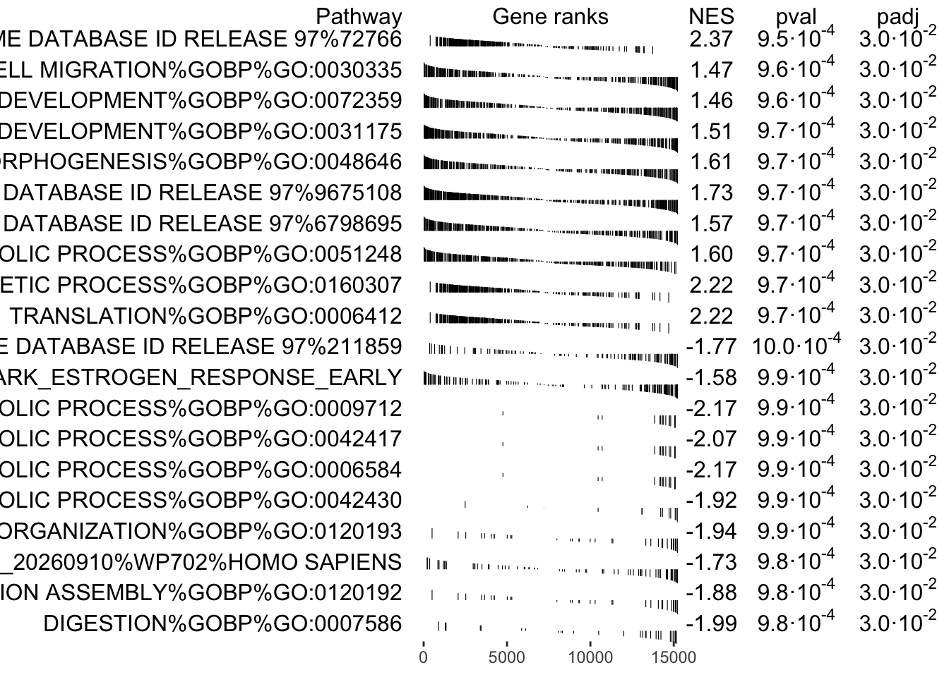

When examining the results there are a few things to look for:

Check the number of gene-sets that have been used for the analysis.

A small number (a few hundred genesets if using baderlab genesets) could indicate an issue with identifier mapping.

Check the number of sets that have FDR less than 0.25 – in order to determine what thresholds to start with when creating the enrichment map. It is not uncommon to see a thousand gene sets pass the threshold of FDR less than 0.25. FDR less than 0.25 is a very lax threshold and for robust data we can set thresholds of FDR less than 0.05 or lower.

Number of pathways with corrected pvalue < 0.05

length(which(fgseaRes$padj < 0.05))

## [1] 325

Number of pathways with corrected pvalue < 0.01

length(which(fgseaRes$padj < 0.01))

## [1] 0

Number of Palbo-resistant (up -regulated) pathways with corrected pvalue < 0.05

length(which(fgseaRes$padj < 0.05 & fgseaRes$ES > 0))

## [1] 297

Number of Parental (down -regulated) pathways with corrected pvalue < 0.05

length(which(fgseaRes$padj < 0.05 & fgseaRes$ES < 0))

## [1] 28

Step 4 - Explore the tabular format of the results

Palbo-resistant (up-regulated genes)

topPathwaysUp <- fgseaRes[ES > 0][head(order(pval), n=5), pathway]

top_palbo_hits <- fgseaRes[which(fgseaRes$pathway %in% topPathwaysUp),]

#format the pathway name colum so that it is easier to see the whole table
top_palbo_hits$pathway <- substr(top_palbo_hits$pathway, start = 1, stop=35)

kable(head(top_palbo_hits), caption = "Top Palbo-resistant pathways") %>%
kable_styling(bootstrap_options = c("striped", "condensed"), font_size = 10)

Table 7: Table 8: Top Palbo-resistant pathways

pathway	pval	padj	ES	NES	nMoreExtreme	size	leadingEdge
TRANSLATION%REACTOME DATABASE ID RE	0.0009524	0.0297521	0.5492339	2.367385	0	338	EEF1A2, ….
POSITIVE REGULATION OF CELL MIGRATI	0.0009615	0.0297521	0.3432083	1.470604	0	324	CAV1, SE….
NEURON PROJECTION DEVELOPMENT%GOBP%	0.0009671	0.0297521	0.3491317	1.507575	0	355	ADGRB1, ….
CIRCULATORY SYSTEM DEVELOPMENT%GOBP	0.0009615	0.0297521	0.3364867	1.456819	0	361	CAV1, SE….
ANATOMICAL STRUCTURE FORMATION INVO	0.0009690	0.0297521	0.3734785	1.610247	0	345	COL6A1, ….

Parental (down-regulated genes)

topPathwaysDown <- fgseaRes[ES < 0][head(order(pval), n=5), pathway]

top_parental_hits <- fgseaRes[which(fgseaRes$pathway %in% topPathwaysDown),]

#format the pathway name colum so that it is easier to see the whole table
top_parental_hits$pathway <- substr(top_parental_hits$pathway, start = 1, stop=35)

kable(head(top_parental_hits), caption = "Top Parental pathways") %>%
kable_styling(bootstrap_options = c("striped", "condensed"), font_size = 10)

Table 9: Table 10: Top Parental pathways

pathway	pval	padj	ES	NES	nMoreExtreme	size	leadingEdge
METAPATHWAY BIOTRANSFORMATION PHASE	0.0009843	0.0297521	-0.4964079	-1.728867	0	68	CYP2J2, ….
TIGHT JUNCTION ORGANIZATION%GOBP%GO	0.0009872	0.0297521	-0.6351792	-1.936928	0	33	GRHL2, M….
INDOLE-CONTAINING COMPOUND METABOLI	0.0009881	0.0297521	-0.7990183	-1.920113	0	13	KYNU, QP….
DIGESTION%GOBP%GO:0007586	0.0009804	0.0297521	-0.6713526	-1.987560	0	29	AKR1C2, ….
TIGHT JUNCTION ASSEMBLY%GOBP%GO:012	0.0009833	0.0297521	-0.6194630	-1.878603	0	32	GRHL2, M….

Step 5 - Visualize the top results

Visualize the top results as different sorts of plots, as demonstrated in the first part of the lab.

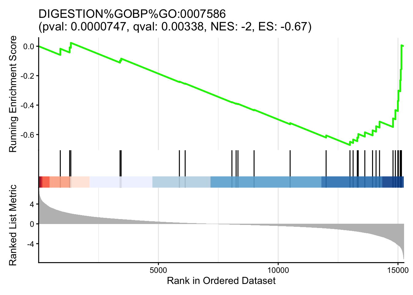
GSEA style Enrichment Plots

In order to create GSEA Enrichment plots we need to use the packages:

• clusterProfiler and
• enrichplot

clusterProfiler runs with its own set of pathways that it parses from GO or KEGG or MSigDB or other sources that are coded into the package. It does not take as input the standard GMT file. If you want to use your own pathway definitions you need to translate it into a dataframe where for every gene in a given pathway there is a row with the pathway name and the gene.

In order to generate an enrichment plot with enrichplot we need the fgsea results in the datastructure returned by clusterProfiler. To run fGSEA in this way we need:

• the ranks file, as before
• the pathways as a data frame.

Below we show how to run fGSEA using the clusterProfiler package and user supplied pathway definitions.

#translate our gmt file (a named list of genesets) into a dataframe
#with one row per gene in each pathway.
TERMS <- data.frame(
    name = rep(names(pathways), lengths(pathways)),
    gene = unlist(pathways, use.names = FALSE)
  )

# specify the gene ranks, and make sure it is in descending order.
gsea_scores <- ranks
gsea_scores <- gsea_scores[!is.na(gsea_scores)]
gsea_scores <- sort(gsea_scores, decreasing = TRUE)

# Set a seed for reproducibility
set.seed(123)

#Run fgsea using clusterProfiler, with the same gene-set size limits as above.
selected_gsea <- clusterProfiler::GSEA(
    geneList = gsea_scores,
    TERM2GENE = TERMS,
    minGSSize = 10,
    maxGSSize = 500,
    pvalueCutoff = 1,
    verbose = FALSE,
    pAdjustMethod = "fdr",
    scoreType = "std",
    eps = 0
  )

## Warning in prepare_gsea_inputs(geneList, scoreType, exponent): There are ties
## in the preranked stats (0.01% of the list). The order of those tied genes will
## be arbitrary, which may produce unexpected results.

Print out a few of the top enrichment plots

all_figures <- list()

#generate GSEA plots for the top Parental (down-regulated) genesets that we have already seen in the table above
rows_to_use <- which(selected_gsea@result$ID %in% topPathwaysDown)

for(i in seq_along(rows_to_use)){
  row_number = rows_to_use[i]

  #format the title for the enrichment plot
  pw_des <- selected_gsea@result$Description[row_number]
  pw_pval <- selected_gsea@result$pvalue[row_number]
  pw_pval <- format(pw_pval, scientific = F, digits = 3)
  pw_qval <- selected_gsea@result$p.adjust[row_number]
  pw_qval <- format(pw_qval, scientific = F, digits = 3)
  pw_nes <- selected_gsea@result$NES[row_number]
  pw_nes <- format(pw_nes, scientific = F, digits = 2)
  pw_es <- selected_gsea@result$enrichmentScore[row_number]
  pw_es <- format(pw_es, scientific = F, digits = 2)
  mytitle <- glue::glue('{pw_des}\n(pval: {pw_pval}, qval: {pw_qval}, NES: {pw_nes}, ES: {pw_es})')


  figure <- enrichplot::gseaplot2(
    selected_gsea,
    geneSetID = selected_gsea@result$ID[row_number],
    title = mytitle,
    color = "green2",
    base_size = 12,
    rel_heights = c(1.5, 0.5, 1),
    subplots = 1:3,
    pvalue_table = F,
    ES_geom = "line"
  )

  all_figures[[i]] <- figure
}

#display the first 3 enrichment plots
for (figure in head(all_figures, 3)) {
  print(figure)
}

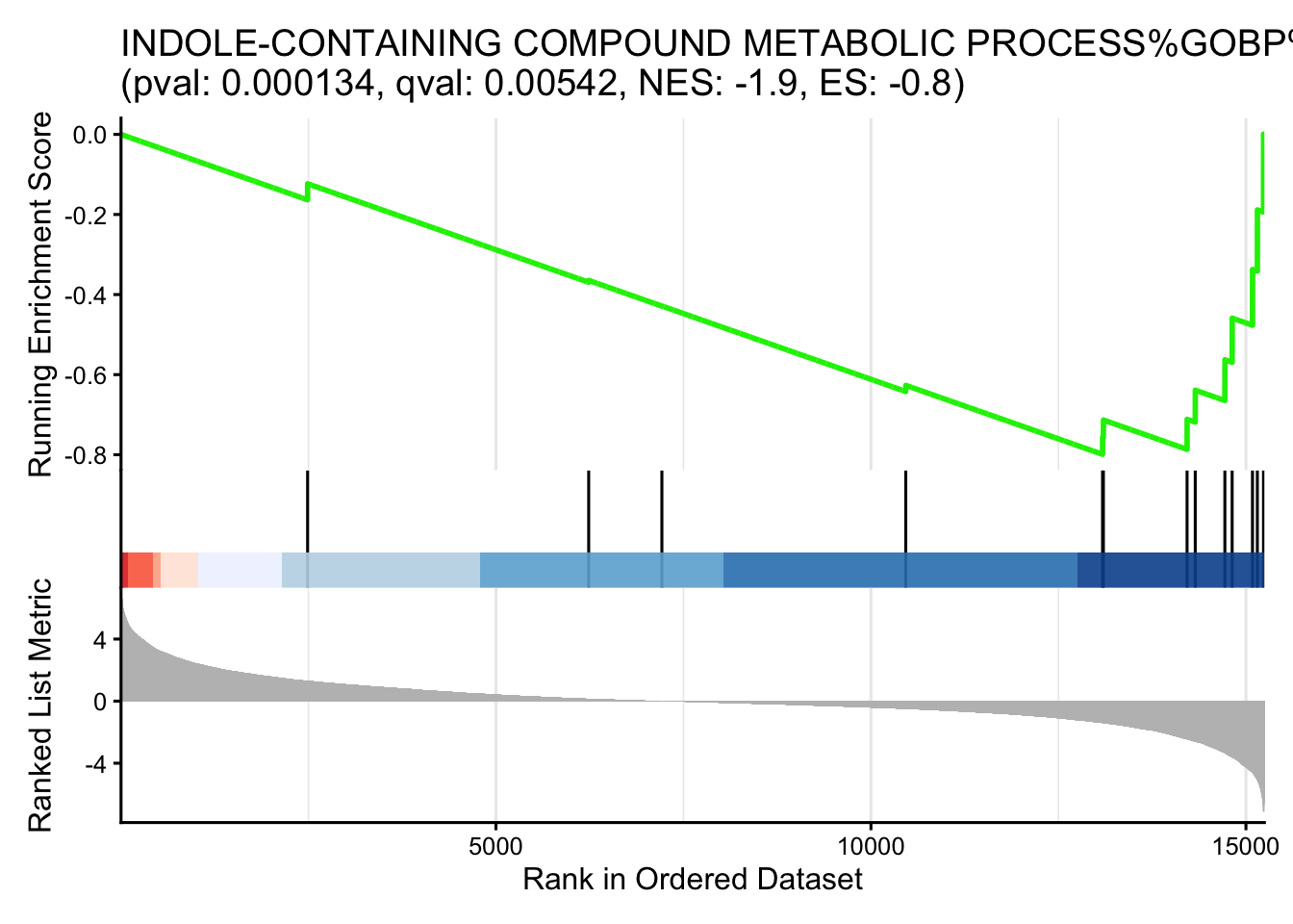
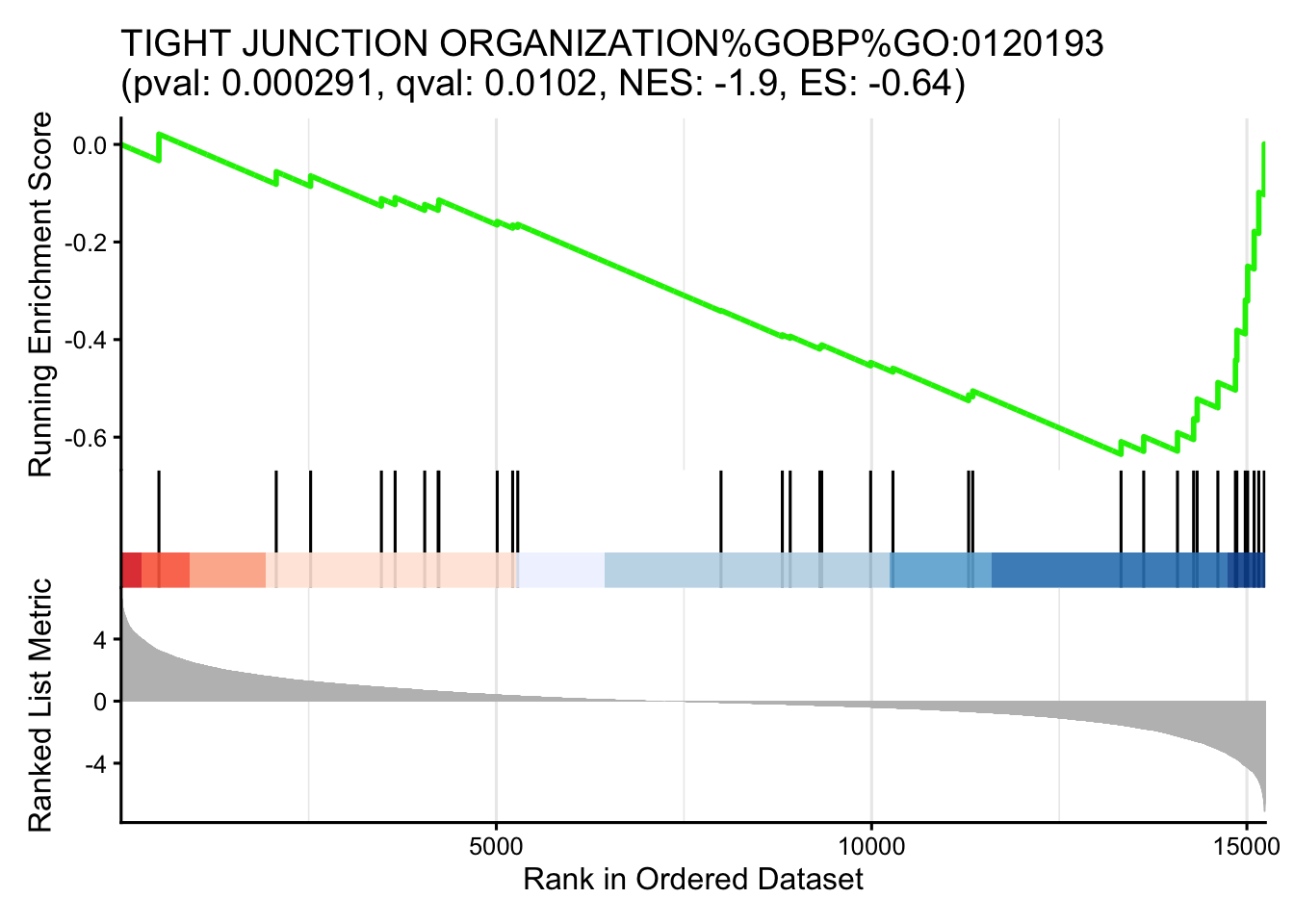
Bar plots

• top pathways associated with Parental

topPathwaysDown <- fgseaRes[ES < 0][head(order(pval), n=20), pathway]

enrichment_results_topdown <- fgseaRes[which(fgseaRes$pathway %in% topPathwaysDown),]

#change the name to be just the first part of the name
enrichment_results_topdown$pathway <- unlist(lapply(enrichment_results_topdown$pathway, FUN=function(x){unlist(strsplit(x,split = "%"))[1]}))
#make sure that names are unique after shortening them (the same name can come from different databases)
enrichment_results_topdown$pathway <- make.unique(enrichment_results_topdown$pathway)

##Calculate a score: the absolute value of the NES.
##(the pvalues of the top pathways are all very close to each other, so the NES is more informative here)
enrichment_results_topdown$score = abs(enrichment_results_topdown$NES)

enrichmentTidy <- enrichment_results_topdown %>%
  as_tibble() %>%
  arrange(desc(score)) %>%
  slice_head(n = 20)

p = ggplot(enrichmentTidy, aes(reorder(pathway, score), score)) +
  geom_col(aes(fill = score), width=0.8) +
  scale_fill_gradient(low = "#C1F6F8", high = "#00BFC4")+
  coord_flip() +
  labs(x="", y="Normalized Enrichment Score (absolute value)",
       title="Pathway enrichment analysis - \nParental") +
  theme_minimal()

p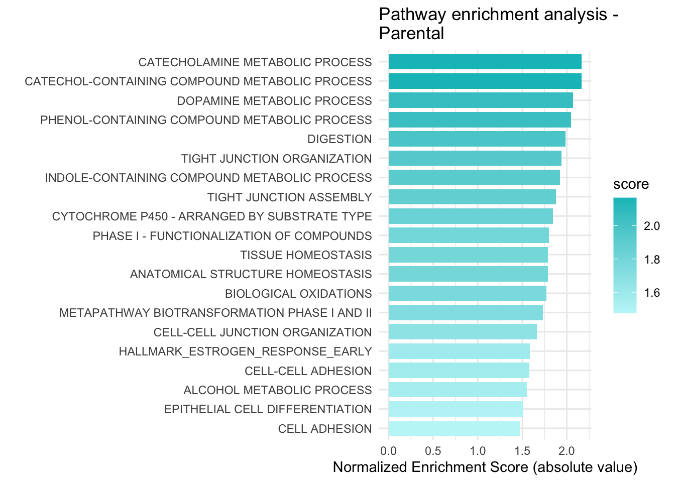

##YOUR TURN##

## Generate the same bar plot for the top 20 Palbo-resistant results.
## Change the colour of the bars to a different colour as
## they are a different phenotype than the Parental set.

Dot plot

• top pathways associated with Parental

p = ggplot(enrichment_results_topdown, aes(
  y = fct_reorder(pathway, score),
  x = score,
  color = score,
  size = size
)) +
  geom_point() +
  scale_color_gradientn(
    colours = c("lightpink", "lightblue", "blue"),
    guide = guide_colorbar(reverse = FALSE, order = 1)
  ) +
  scale_size_continuous(range = c(4, 8), name = "genes in set") +
  theme_bw(base_size = 12) +
  xlab("Normalized Enrichment Score (absolute value)") +
  ylab(NULL) +
  ggtitle("Pathway Enrichment Analysis - \n Parental") +
  theme(
    axis.text.y = element_text(size = 7)
  )
p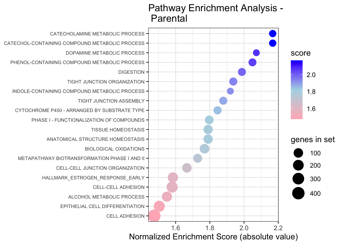

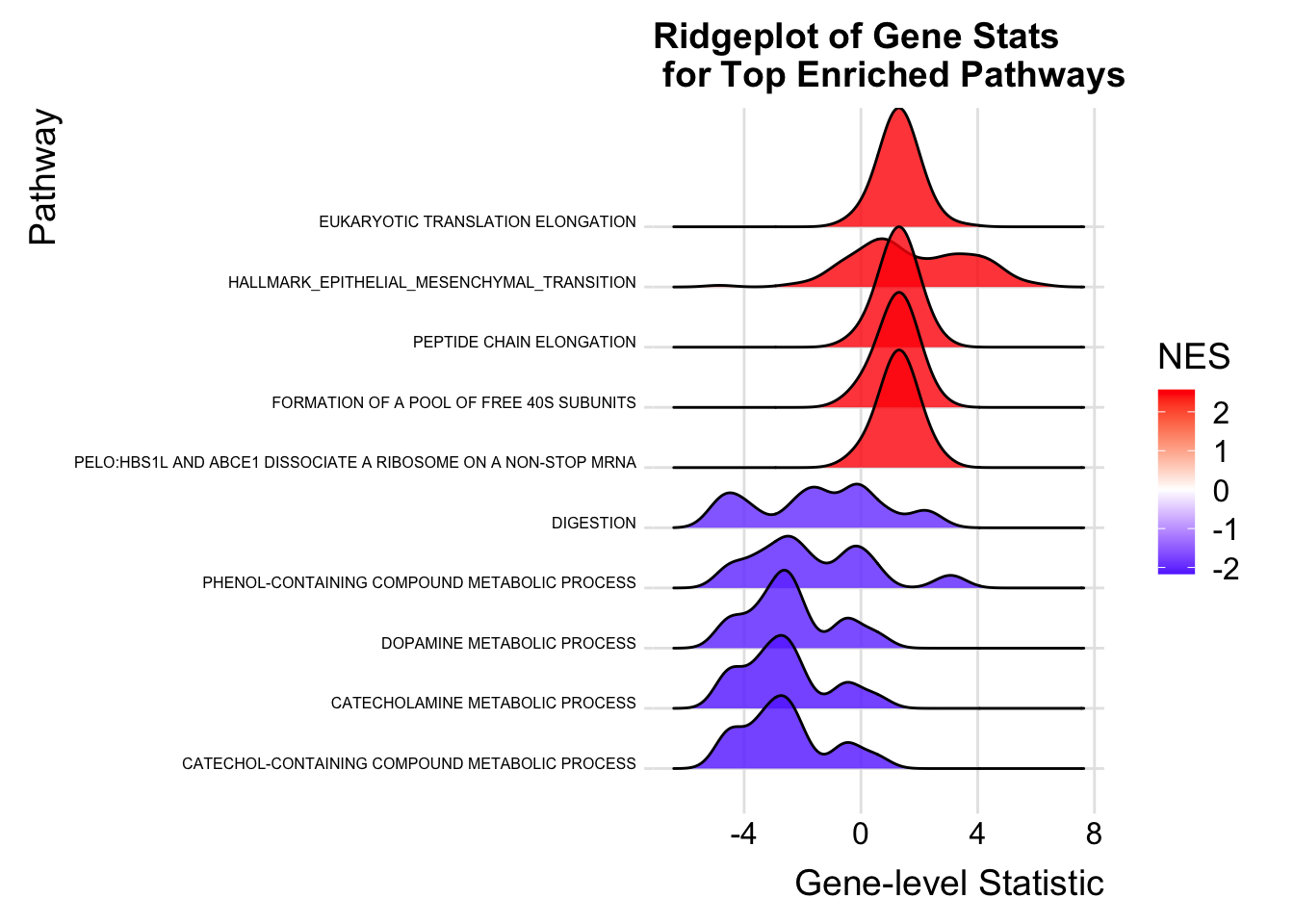
##YOUR TURN##

## Generate the same dot plot for the top 20 Palbo-resistant results.
## Change the colour of the dots to a different colour range as
## they are a different phenotype than the Parental set.

Ridge plots

• top pathways associated with either class

# Filter significant pathways (adjusted p-value < 0.05) and take
# the top 5 for each class (highest positive NES and most negative NES)
significant_pathways <- fgseaRes[padj < 0.05]
topPathways <- rbind(
  head(significant_pathways[NES > 0][order(-NES)], 5),
  head(significant_pathways[NES < 0][order(NES)], 5)
)

# Create a data.frame for plotting with the gene ranks for each of the top pathways
ridge_data <- rbindlist(lapply(topPathways$pathway, function(pw) {
  genes <- pathways[[pw]]
  data.frame(
    gene = genes,
    stat = ranks[genes],
    pathway = pw
  )
}))


# get NES for each of the top pathways
nes_map <- setNames(topPathways$NES, topPathways$pathway)

# Add NES values to ridge_data
ridge_data$NES <- nes_map[ridge_data$pathway]

#change the name to be just the first part of the name (because the actual names are too long)
#and make sure that names are unique after shortening them
short_names <- make.unique(unlist(lapply(topPathways$pathway, FUN=function(x){unlist(strsplit(x,split = "%"))[1]})))
names(short_names) <- topPathways$pathway
ridge_data$pathway <- short_names[ridge_data$pathway]

#get rid of na values for genes found in the gene set but not ranked in our dataset.
ridge_data <- ridge_data[!is.na(ridge_data$stat),]

ggplot(ridge_data, aes(x = stat, y = reorder(pathway, NES), fill = NES)) +
  geom_density_ridges(scale = 2, alpha = 0.8) +
  scale_fill_gradient2(
    low = "blue", mid = "white", high = "red", midpoint = 0,
    name = "NES"
  ) +
  theme_ridges() +
  theme(legend.position = "right",axis.text.y = element_text(size = 6)) +
  labs(
    title = "Ridgeplot of Gene Stats\n for Top Enriched Pathways",
    x = "Gene-level Statistic",
    y = "Pathway"
  )

NOTE: In the next module, you will learn a better approach to address redundancy and visualize enriched gene sets as networks using Cytoscape and EnrichmentMap.